Argo Canada BGC Quality Control

general description

A python library of functions for quality controlling dissolved oxygen data. Heavily based on the SOCCOM BGC Argo QC methods program in matlab, uses either NCEP or World Ocean Atlas data to calculate oxygen gains (Johnson et al. 2015).

installation

The recommended install is through the conda-forge channel, via the command:

conda install -c conda-forge bgcArgoDMQC

The package is also available through the python package index https://pypi.org/project/bgcArgoDMQC/, install with:

pip install bgcArgoDMQC

dependencies

Must run on python3.4 or higher, not supported on python2.x (uses pathlib, introduced in python version 3.4)
TEOS-10 package gsw
netCDF4 module for .nc files
pandas is required
seaborn
cmocean is recommended for nicer plots, but not required

setup

This package uses locally saved data, as it is designed for QC operators that will likely want to manipulate or export files. This includes accessing WOA and NCEP data. Therefore, the user must tell the package where to look for data. This can either be done inline using the function bgc.set_dirs(...), or permanently using the following code:

from bgcArgoDMQC.configure import configure

argo_dir = '/path/to/my/argo/data/'
woa_dir  = '/path/to/woa/data/'
ncep_dir = '/my/ncep/path/

configure(argo_path=argo_dir, woa_path=woa_dir, ncep_path=ncep_dir)

Other items like operator_name and operator_orcid can be set in this matter as well to a .config file saved where the package exists on your machine. All required Argo and reference data can be downloaded using the io component of the package, see documentation for more details. All data paths should be structured as they are found. For example, the Argo path should follow the dac structure, so in this example, a profile might be found in '/path/to/my/argo/data/dac/meds/4900869/profiles/BR4900869_024.nc'.

basic functionality

This section will show the two main components of DOXY DMQC, visually inspecting the data, and calculating the gain relative to a reference dataset. There are many more visualizations that are possible, refer to docs for full plotting reference.

# import package
import bgcArgoDMQC as bgc

# define a WMO number you want to look at
wmo = 4900869
# load into a synthetic profile object
syn = bgc.sprof(wmo)
# look at the current state of QC flags for T, S, and DO
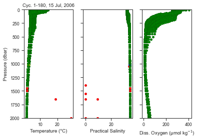
g1 = syn.plot(kind='qcprofiles', varlist=['TEMP', 'PSAL', 'DOXY'])

We can see above that most T/S points are good, with a few obvious outliers in red. The oxygen data also look all good. This is an old float, but for current floats the QC flag for unadjusted oxygen should be 3 (probably bad).

Since this is an older float, there are no in-air measurements made by the optode. Therefore we will calcualte the gain by comparing surface values to WOA data.

# calculate the gains
gains = syn.calc_gains(ref='WOA')

The ref keyword argument sets the reference dataset. In this case we set it to WOA data. By default ref is set to 'NCEP', but in this case that would return all NaN values since there is no in-air data for this float.

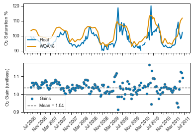
Visualize the gains in a single line:

# plot gains over time, show source data
g3 = syn.plot('gain', ref='WOA')

I find this plot particularly useful, as sometimes it is a good indicator to go back and inspect certain profiles. We see a couple large spikes in the suface float data. Are those spikes real, or should we go back and have a closer look at those profiles? This could change our mean gain a little, and perhaps we would flag some data as bad that we didn't notice before.

future developments

improved netcdf exporting
gain calculation with drift, surface carryover for in-air gains
expanded capabilities for DMQC on other BGC variables
data access via internet (through a package like argopy or argopandas)