Brickman

Convenience tools for accessing Brickman Gulf of Maine 2050 model outputs.

Cf: Brickman D, Alexander MA, Pershing A, Scott JD, Wang Z. Projections of physical conditions in the Gulf of Maine in 2050. Elem Sci Anth. 2021 May 6;9(1):00055.

Contents:

PRESENT CLIMATE
RCP45
- year 2055
- year 2075
RCP85
- year 2055
- year 2075

Variables:

Bathy_depth, land_mask
Annual means: SST, MLD, SSS, Sbtm, Tbtm, U, V, Xbtm
Monthly means: SST, MLD, SSS, Sbtm, Tbtm, U, V, Xbtm

Requirements

Installation

remotes::install_github("BigelowLab/brickman")

Usage

Reading and plotting

suppressPackageStartupMessages({
    library(stars)
    library(brickman)
    library(sf)
    library(dplyr)
    library(tidyr)
    library(ggplot2)
  })

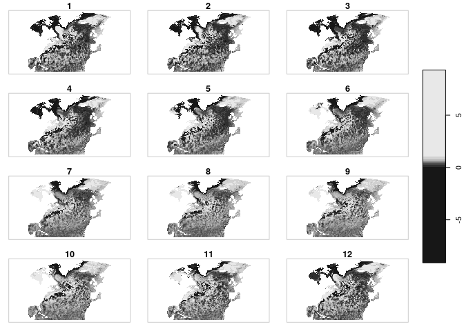
x <- brickman::read_brickman(scenario ='RCP85', year = 2055, vars = 'SST', interval = "mon")
plot(x)

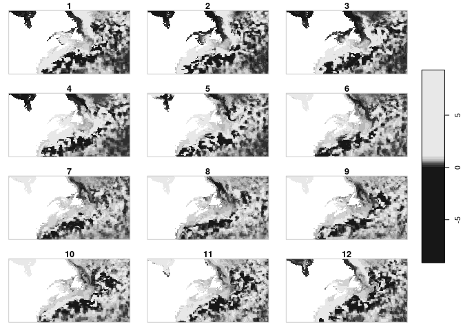
Plotting a portion of curvilinear grid

You can display a portion of a curvilinear grid by specifying the drawing extent. Note that by default R expands the plotting region. The orange box shows the extent of the bounding box we used to define the extent.

bb = c(xmin = -77, ymin = 36.5, xmax = -42.5, ymax = 56.7) |>
  st_bbox(crs = st_crs(x)) 
box = st_as_sfc(bb)  
plot(x, 
     extent = bb, 
     reset = FALSE,
     axes = FALSE)

## downsample set to 5

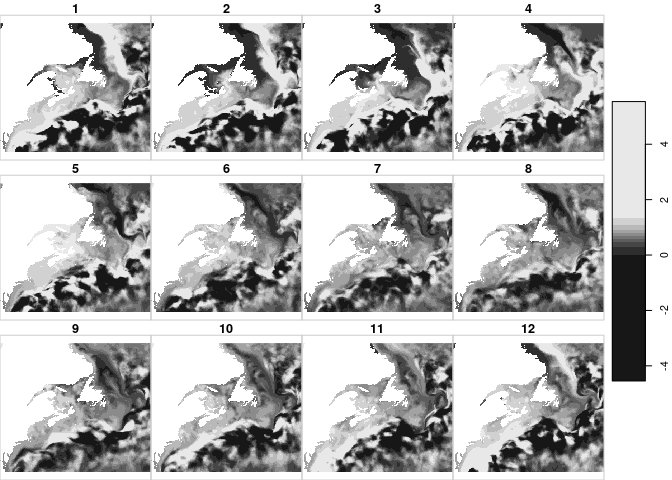
plot(box, color = NA, border = "orange", add = TRUE)

Subsetting/Cropping by transforming to regular grid

Subsetting and cropping curvilinear grid is not supported by stars because (I think) gdal doesn’t support it. We can transform (warp) to a regular grid and then subset.

box4326 = st_transform(box, 4326)
warped = warp_brickman(x, crs = sf::st_crs(box4326))
sub = warped[bb]
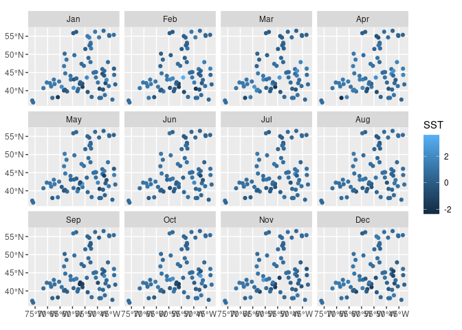
plot(sub, reset = FALSE)

Extracting

Points can be extracted easily from the regular grid.

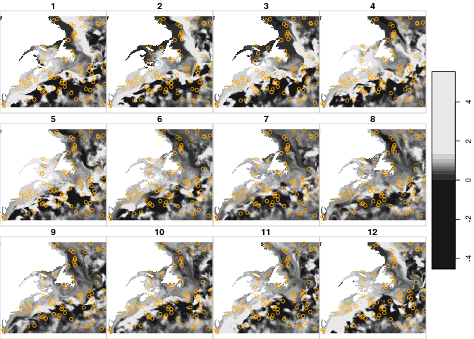
points = sf::st_sample(sf::st_as_sfc(bb), 100)

px = stars::st_extract(warped, points) |>
  sf::st_as_sf() |>
  rlang::set_names(c(month.abb, "geometry")) |>
  tidyr::pivot_longer(where(is.numeric),
                      names_to = "month",
                      values_to = "SST") |>
  dplyr::mutate(mon = match(month, month.abb)) |>
  dplyr::filter(!is.na(SST))


plot_hook = function(..., row = 0, col = 0, nr = 0, nrow = 0, ncol = 0, value = 0, bbox = NULL) {
  #cat("nr = ", nr, class(nr), "\n")
  z = dplyr::filter(px, mon == nr)
  plot(z['SST'], col = "orange", add = TRUE)
}

plot(sub, hook = plot_hook)

px = px |>
  dplyr::mutate(month = factor(month, levels = month.abb)) 
ggplot() +
  geom_sf(data = px, aes(colour = SST)) +
  facet_wrap(~month)