Here, we outline the re-analysis of two GEO datasets, GSE100579 and GSE131972, both of which are investigating the effect of acute stress on the translatome (TRAP-seq) of CA3 pyramidal neurons in the mouse hippocampus. The exact annotation of the samples is available at here.
These datasets were used for three separate publications:
- Marrocco J. et al. 2017; A sexually dimorphic pre-stressed translational signature in CA3 pyramidal neurons of BDNF Val66Met mice; Nature Communications volume 8, Article number: 808 (2017)
- Gray J. D. et al. 2018; Translational profiling of stress-induced neuroplasticity in the CA3 pyramidal neurons of BDNF Val66Met mice; Molecular Psychiatry volume 23, pages 904–913
- Marrocco J. et al. 2019; Early Life Stress Restricts Translational Reactivity in CA3 Neurons Associated With Altered Stress Responses in Adulthood; Front. Behav. Neurosci.
We show that a number of the analyses and claims made in these publications are well not supported by the data and not reproducible across the two datasets. The use of appropriate statistical methods to uncover interactions fails to demonstrate significant sexually dimorphic or early-life-dependent responses to stress, highlighting the fact that these studies were underpowered to address such questions.
We acquired the deposited raw sequencing fastq files from the online repositories GSE100579 (10 sequencing runs for (Marrocco et al. 2017, Gray et al. 2018) and GSE131972 (sequencing 10 runs for (Marrocco et al. 2019)) and used kallisto (DOI:10.1038/nbt.3519, version 0.44.0) for the pseudoalignment of reads on the GENCODE M17 transcriptome, with an estimated fragment length of 200 ±20. However, we also reproduced the full analysis using a transcriptome-based analysis as the authors did in some of the publications.
We first load the necessary packages and the data:
library(edgeR)
library(SEtools)
library(SummarizedExperiment)
library(sva)
library(DESeq2)
source("misc.R")
kallistodata <- readRDS("data/AllData.kallisto.SE.rds")
set.seed(12345)
Because we later provide a meta-analysis of the datasets, we will work on a uniform, kallisto-based quantification. However, the re-assessment of the authors' original claims were also reproduced using an alternative quantification method (see codingTranscriptome.md).
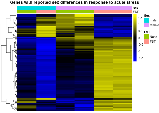
In the 2017 publication the authors report that numerous genes are differentially regulated between males and females after acute stress. Unfortunately, they do not include a list with all genes in the publication, but Table 1 contains a subsets of genes that are reported as differentially regulated between males and females upon acute stress (forced swim test - FST). First, we inspect the expression pattern of these genes across the runs used in the original publication in WildType animals:
se <- kallistodata
se <- subset(se,select  = se$Set == "GSE100579" & se$Genotype == "WildType")
genes <- read.table("metadata/Marrocco2017GenderStressGenes.csv", sep = ";", header = T)$genes
se <- se[,order(se$Sex,se$FST)]
sehm(se, genes, do.scale=T, assayName="logcpm", anno_columns=c("FST","Sex"),
     cluster_rows = T, main = "Genes with reported sex differences in response to acute stress")
Rows in the plot represent the reported genes, while the columns are samples, and the colors represent variance-scaled log-normalized expression values (i.e. row z-scores). From this plot, it indeed looks like these genes have a very different response to FST in males and females. However, 6 independent samples is insufficient to investigate 4 experimental groups.
The same study also includes males and females from a different genotype (BDNF mutants) exposed to stress, and we can inspect the behavior of those genes in these additional samples:
se <- kallistodata
se <- subset(se,select  = se$Set == "GSE100579")
se <- se[,order(se$Genotype,se$Sex,se$FST)]
sehm(se, genes, do.scale=T, assayName="logcpm", anno_columns=c("FST","Sex","Genotype"),
     cluster_rows = T, main = "Genes with reported sex differences in response to acute stress",
     gaps_at = "Genotype")
We here observe that the BDNF mutant males appear to have an expression pattern, for the reported genes, which mimics the wildtype females, while the mutant females not exposed to stress have an expression pattern, for those genes, which resembles that of stressed wildtype females. While it is possible that the mutation entirely reverses the expression pattern of thoses genes, most groups are represented by a single sample, and an arguably more likely explanation would be that these co-expressed genes are the result of random variation unrelated to the experimental variables. To test this, we can include the second dataset (GSE131972):
se <- kallistodata
se <- subset(se,select  = se$ELS == "None" & se$Genotype == "WildType")
se <- se[,order(se$Set,se$Sex,se$FST)]
sehm(se,genes,do.scale = T,anno_columns = c("FST","Sex","Set"), gaps_at = "Set", cluster_rows = T, main =  "Same genes in wild-type samples, including the dataset")
## Using assay logcpm
Although the second dataset includes only males, one can immediately notice that, upon stress and with respect to the aforementioned genes, some of the males behave exactly like the males of the first dataset, while others behave exactly like females. It becomes clear, therefore, that these genes are co-expressed and highly variable across all samples, independently of sex.
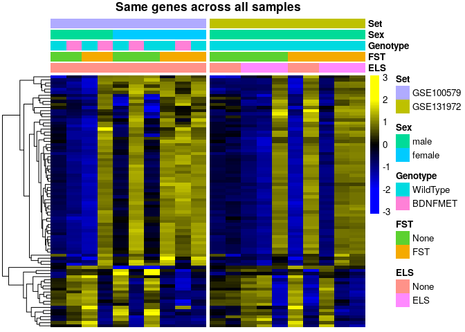
If we further visualize these genes across all samples, we find
se <- kallistodata
se <- se[,order(se$Sex,se$FST)]
sehm(se, genes, do.scale=T, assayName="logcpm", cluster_rows = T, gaps_at = "Set",
     anno_columns=c("ELS","FST","Genotype","Sex","Set"), main="Same genes across all samples")
The high co-expression of the reported genes suggests that the variability is the result of a single vector of variation, which could be technical, but is in any case unrelated to the experimental design. To investigate this, we attempt to model this vector of variation using Surrogate Variable Analysis (SVA - see the exact implementation here), and to visualize the reported genes in the corrected data:
se <- dosvacor(se, form = ~ Set + Sex * FST, form0 = ~Set)## converting counts to integer mode
## Number of significant surrogate variables is:  2
## Iteration (out of 5 ):1  2  3  4  5
sehm(se, genes, do.scale=T, assayName="corrected", anno_columns=c("ELS","FST","Genotype","Sex","Set"),
     cluster_rows=T, main="Same genes after correcting for technical variability")
As we can see, removing technical variability abolishes the effects for the male-female stress difference seen in the single replicate comparisons.
Together, this re-analysis indicates that the reported sex-specific transcriptional responses to stress are not supported by the data.
A complete assessment of the findings of Gray et al. 2018 is unfortunately not possible since the repository GSE100579 is missing critical samples for the chronic stress model for the BDNF Val66Met genotype and only includes samples of acute stress.
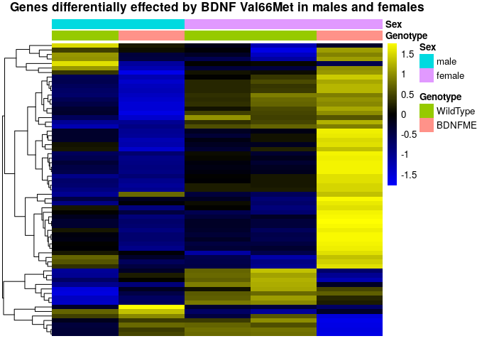
However, the authors claim that many genes are differentially regulated between WildType and BDNF Val66Met animals at baseline, a regulation which is dependent on sex. While no complete list of genes has been included in the publication, a subset can be found in the publication's Table 1.
We plot these genes in the GSE100579 data set:
se <- kallistodata
genes <- read.table("metadata/Gray2018GenotypeGenes.csv", sep = ";", header = T)$genes
se <- subset(se,select  = se$Set == "GSE100579" & se$FST == "None")
se <- se[,order(se$Sex,se$Genotype)]
sehm(se, genes, do.scale=T, assayName="logcpm", anno_columns=c("Genotype","Sex"), cluster_rows=T,
     main="Genes differentially effected by BDNF Val66Met in males and females")
Again, we find that the experimental design was severly underpowered. We investigate the expression of these genes across all samples from both datasets.
se <- kallistodata
se <- se[,order(se$Sex,se$Genotype,se$FST)]
sehm(se, genes, do.scale=T, assayName="logcpm", anno_columns=c("FST","Genotype","Sex"), cluster_rows=T,
     main="Same genes across all samples")
We see a similar pattern as for the differences reported in Marrocco et al 2017: the baseline difference cannot be reproduced in the additional samples, where these genes instead show high intra-group variability.
As described above, we again eliminate technical variabilty and re-visualize the same genes:
se <- dosvacor(se, form = ~Set + Sex + Genotype + FST + ELS, form0 = ~Set)## converting counts to integer mode
## Number of significant surrogate variables is:  3
## Iteration (out of 5 ):1  2  3  4  5
sehm(se, genes, do.scale = T,anno_columns = c("FST","Genotype","Sex","Set"), cluster_rows = T,assayName = "corrected", main = "Same genes after removing technical variabilty")It becomes apparent that these genes were again the result of variation unrelated to the experimental groups, and that the vast majority of them do not show genotype-dependent differences between males and females at baseline.
Here we re-analyse Marrocco et al. 2019 checking for early life stress (ELS) -dependent changes in the acute stress (AS) response. The results presented here are also largely reproduced using a different quantification and using DESeq2 instead of edgeR. Although DESeq2 produced a few more hits, all analyses had similar results, and the core message of the original publication, namely that ELS substantially impacts the transcriptional acute stress response, could not be reproduced with either method.
se <- kallistodata
se <- se[order(rownames(se)),]
se <- subset(se,select  = se$Set == "GSE131972")
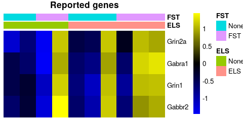
In their publications the authors unfortunately do not upload a list with differentially expressed genes. However, in their discussion they mention a number of genes that they thought to be differentially expressed between ELS and non-ELS mice after acute stress. We look at the expression of these genes across the very samples used in their study. They claim that selected genes are only induced in non-ELS mice following FST:
sehm(se, c("Grin1","Grin2a","Gabbr2","Gabra1"), do.scale=T, assayName="logcpm",
     anno_columns = c("ELS","FST"),  main = "Reported genes")
In light of the very large intra-group variability of these genes, it appears unlikely that these genes are indeed only induced in non-ELS treated mice.
Further, they claim that a restricted set of genes is selectively induced by FST in ELS mice but not non-ELS mice.
sehm(se, c("Per1", "Npy", "Nfkbia", "Penk","Dusp1", "Cst3", "Trib1", "Htra1", "Sdc4", "Plekhf1"), do.scale=T, assayName="logcpm", anno_columns = c("ELS","FST"), main = "Reported genes")While these genes might be increased in expression in ELS mice upon stress, the variability across samples of the same group prevents strong claims. In particular, the claim that these genes are not activated in the non-ELS group appears questionable, as one of the two non-ELS samples shows an activation of these genes. More refined analysis (see below), as well as a larger sample size, would be needed to address this question with confidence.
Finally, the authors claim that there are a number of genes that appear to be induced by AS in both ELS and non ELS mice, including the following:
sehm(se, c("Egr1", "Egr2", "Egr4", "Arc","Fos", "Fosb"), do.scale=T, assayName="logcpm", anno_columns = c("ELS","FST"), main = "Reported genes")For these well-known genes, indeed, all samples show a consistent increase in response to AS.
To establish whether ELS does impact the translational response to acute stress, the authors analyzed the two response separately and substracted the sets of significant genes. While this practice is widespread, the appropriate analysis is a linear regression using an interaction term, which is fortunately possible using edgeR's generalized linear models. Here we use the standard glmLRT which is less stringent and more susceptible to type 1 errors, but has a better sensitivity in low replicate experiments (an analysis with a glmQL model did not yield any significant results).
#experimental design, interactive model
design <- model.matrix(~se$FST * se$ELS) # identicial to ~FST+ELS+FST:ELS

y <- DGEList(counts=assays(se)$counts)
y <- calcNormFactors(y)
y <- estimateDisp(y,design)
y <- y[filterByExpr(y, design),]

Results <- list()
fit <- glmFit(y,design)
for(i in colnames(design)[-1]){
  Results[[i]] <- glmLRT(fit, i)
}
We first ask whether that are genes altered by acute stress:
topTags(Results$`se$FSTFST`)## Coefficient: se$FSTFST
## logFC logCPM LR PValue FDR
## Nadsyn1 7.788697 -0.1856326 23.30605 1.381649e-06 0.02027432
## Fos 2.092030 5.1006405 18.81602 1.439529e-05 0.06223390
## Egr4 1.608956 5.8854438 18.63037 1.586727e-05 0.06223390
## Plekhg3 -2.202026 2.4615140 18.50292 1.696440e-05 0.06223390
## Fosb 1.899855 4.4234011 17.92003 2.303836e-05 0.06761298
## Stard9 -4.217794 -0.4341469 14.86158 1.156958e-04 0.28295333
## Mill2 4.024261 -1.3626955 14.07301 1.758488e-04 0.36862931
## Egr2 2.233255 2.4233386 13.55050 2.322299e-04 0.42596774
## RP23-62O7.9 -7.148746 -1.2582485 13.13874 2.892520e-04 0.47160925
## Ushbp1 -6.790005 -1.5724706 12.53551 3.992913e-04 0.58592012
Even though the data looked promising only one gene passes mutliple testing correction, most likely owing to the insufficient sample size.
We next ask whether there are genes altered by early life stress?
topTags(Results$`se$ELSELS`)## Coefficient: se$ELSELS
## logFC logCPM LR PValue FDR
## Nadsyn1 7.786364 -0.1856326 24.327310 8.127852e-07 0.01192681
## Il10ra -7.357688 -1.1359543 20.922603 4.782183e-06 0.03508688
## Tec -4.488194 -2.3191622 19.189000 1.183937e-05 0.05791029
## Mill2 3.827833 -1.3626955 13.872101 1.956818e-04 0.71785853
## Piga -1.592914 1.5385751 11.174924 8.291030e-04 0.99997057
## RP23-45E20.3 6.234163 -1.4397776 9.676333 1.866568e-03 0.99997057
## Ecel1 -1.884815 -0.1093226 8.877256 2.887451e-03 0.99997057
## Pcdha4 1.080423 3.5528592 8.774824 3.054166e-03 0.99997057
## Lrrc40 0.978220 5.7617445 8.714893 3.156209e-03 0.99997057
## Syt9 -1.434765 1.2125522 8.685376 3.207734e-03 0.99997057
Again, only two genes passe the multiple testing correction.
We finally investigate whether there are genes with a significant interaction:
topTags(Results$`se$FSTFST:se$ELSELS`)## Coefficient: se$FSTFST:se$ELSELS
## logFC logCPM LR PValue FDR
## Nadsyn1 -8.140952 -0.1856326 20.23596 6.845398e-06 0.07496231
## Plekhg3 2.821723 2.4615140 19.21165 1.169970e-05 0.07496231
## Stard9 5.692110 -0.4341469 18.69660 1.532554e-05 0.07496231
## Il10ra 8.307574 -1.1359543 16.67533 4.435416e-05 0.16271322
## Piga 2.638569 1.5385751 14.23779 1.611024e-04 0.47280344
## Ushbp1 7.918531 -1.5724706 13.18878 2.816307e-04 0.68877487
## Mill2 -4.526715 -1.3626955 12.81546 3.437665e-04 0.72063280
## Tle6 -9.289217 -1.9395041 11.65911 6.388886e-04 0.99984358
## RP23-45E20.3 -7.905188 -1.4397776 11.19965 8.181289e-04 0.99984358
## Rpl9-ps6 -12.073767 -2.0080711 11.01066 9.058948e-04 0.99984358
No genes have a altered acute stress response in ELS vs normal animals. This is stark contrast with the authors' conclusions, reporting that hundreds of genes show altered expression in response to FST in ELS vs non-ELS groups.
A similar analysis using DESeq2 instead of edgeR reaches similar conclusions.
Given that the original studies were underpowered, we combined the data from both accessions to try to give more robust answers to the questions raised by the authors, in particular:
- are genes differentially translated following forces swim stress?
- are genes differentially translated following males and females?
- are genes differentially translated in BDNF Val66Met mice?
- are genes differentially translated following early life stress
- are responses of FST genes altered by sex?
- are responses of FST genes altered by BDNF Val66Met?
- are responses of FST genes altered by early life stress?
We first ran an analysis over all data to determine if there are any significant effects for forces swim stress (=FST), Sex, Genotype or early life stress (=ELS). In the process we also remove technical variabilty to increase the chance of successfully finding candidate genes. Here, we use a glmQL model in order to better correct for type I errors.
se <- kallistodata
se <- dosvacor(se, form = ~FST + Sex + Genotype + Set + ELS, form0 = ~Set)
## converting counts to integer mode
## Number of significant surrogate variables is:  3
## Iteration (out of 5 ):1  2  3  4  5
#experimental design, full additive model
design <- model.matrix(~ se$SV1 + se$SV2 + se$SV3 + se$FST + se$Sex +
                         se$Genotype + se$Set + se$ELS )

y <- DGEList(counts=assays(se)$counts)
y <- calcNormFactors(y)
y <- estimateDisp(y,design)
y <- y[filterByExpr(y, design),]

Results <- list()
fit <- glmQLFit(y,design)
for(i in colnames(design)[-1]){
  Results[[i]] <- glmQLFTest(fit, i)
}se <- se[,order(se$FST)]
sehm(se, rownames(topTags(Results$`se$FSTFST`,p.value = 0.05, n = 1000)), assayName = "corrected", do.scale = TRUE, anno_columns=c("ELS","FST","Genotype","Sex","Set"), main="Significant FST genes with corrected data")sehm(se, rownames(topTags(Results$`se$FSTFST`,p.value = 0.05, n = 1000)), assayName = "logcpm", do.scale = TRUE, anno_columns=c("ELS","FST","Genotype","Sex","Set"), main="Significant FST genes with uncorrected data")topTags(Results$`se$FSTFST`, p.value = 0.05, n = 30)## Coefficient: se$FSTFST
## logFC logCPM F PValue FDR
## Egr4 1.3763325 5.69996696 271.17725 2.613587e-11 3.884575e-07
## Fosb 1.5939943 4.22512087 203.03955 2.204849e-10 1.230608e-06
## Egr2 2.5189229 2.25835614 199.75180 2.483902e-10 1.230608e-06
## Sik1 1.0842277 3.49087999 186.74653 4.054620e-10 1.506595e-06
## Fos 2.1424546 4.90675828 157.94276 1.357847e-09 4.036337e-06
## Dusp5 0.9302143 5.63293521 135.24829 4.095570e-09 1.014541e-05
## Nr4a1 1.0909105 6.53490701 111.61093 1.570281e-08 3.334154e-05
## Egr1 0.9829610 8.09783506 107.57296 2.025511e-08 3.381751e-05
## Arc 1.1542530 7.61316750 107.40265 2.047753e-08 3.381751e-05
## Gadd45b 0.7056771 4.63279778 74.25750 2.450426e-07 3.388438e-04
## Junb 0.9275956 6.61596306 73.99547 2.507759e-07 3.388438e-04
## Fosl2 0.4243778 5.91927337 66.78176 4.877095e-07 6.040689e-04
## Arl4d 0.9392704 4.17043954 62.95242 7.114124e-07 7.759527e-04
## Midn 0.4719433 5.65211023 62.68537 7.308980e-07 7.759527e-04
## Ier5 0.4552744 6.35415703 54.11106 1.836552e-06 1.810796e-03
## Maff 1.5236033 -0.09340333 53.59057 1.949320e-06 1.810796e-03
## Per1 0.5599399 6.23132349 51.41371 2.513724e-06 2.197734e-03
## Ier2 0.7775034 3.39046862 50.36234 2.850832e-06 2.353995e-03
## Ppp1r3g 0.8944428 2.92435435 45.80922 5.039660e-06 3.942340e-03
## Spry4 0.4622725 4.09595448 43.02060 7.301071e-06 5.425791e-03
## AC123679.2 -0.6516973 3.46271975 39.62031 1.176666e-05 8.327997e-03
## Sgk1 0.6525801 6.67172638 37.56730 1.593096e-05 1.076281e-02
## Mfsd2a 1.1623871 1.61247631 37.20411 1.682922e-05 1.087533e-02
## Npas4 1.2249991 3.30406700 36.57144 1.853392e-05 1.147790e-02
## Errfi1 0.5098346 6.04496283 35.55216 2.170654e-05 1.290497e-02
## Klf4 1.2173273 -0.05173331 34.75216 2.462893e-05 1.407922e-02
## Oaz3 1.2250014 -0.90753304 33.21588 3.157592e-05 1.738196e-02
## Pim3 0.3712780 5.48950727 32.45968 3.579055e-05 1.899839e-02
## Coq10b 0.3510045 4.95274256 31.89618 3.934544e-05 1.973784e-02
## Trib1 0.6941620 3.45398865 31.57881 4.152221e-05 1.973784e-02
There are multiple candidate genes that are significantly altered by acute stress. Reassuringly, these genes contain many of the well-characterized immediate early genes known to be reliably induced by acute stress challenges (e.g. Egr4, Fos, Dusp1, JunB, Per1, Npas4 etc.).
se <- se[,order(se$Sex)]
sehm(se, rownames(topTags(Results$`se$Sexfemale`,p.value = 0.05, n = 1000)), assayName = "corrected", do.scale = TRUE, anno_columns=c("ELS","FST","Genotype","Sex","Set"), main="Significant sex genes with corrected data")sehm(se, rownames(topTags(Results$`se$Sexfemale`,p.value = 0.05, n = 1000)), do.scale = TRUE, anno_columns=c("ELS","FST","Genotype","Sex","Set"), main="Significant Sex genes with uncorrected data")## Using assay logcpm
topTags(Results$`se$Sexfemale`,p.value = 0.05, n = 30)## Coefficient: se$Sexfemale
## logFC logCPM F PValue FDR
## Ddx3y -12.2457032 4.145685 1279.09472 1.872375e-12 2.782911e-08
## Eif2s3y -11.9705761 3.472145 684.16227 5.086900e-11 3.780330e-07
## Uty -11.2448719 2.663029 414.66507 7.000105e-10 3.468085e-06
## Kdm5d -3.4445982 1.963235 139.38949 3.308488e-09 1.111362e-05
## Prl 14.0460151 3.320776 137.00361 3.738688e-09 1.111362e-05
## Gh 17.7719374 3.429231 87.81891 1.408628e-07 3.489406e-04
## Mthfd1 0.8049886 5.046165 50.59195 2.773064e-06 5.888007e-03
## Fosl2 -0.6841784 5.919273 45.18028 5.470748e-06 1.016397e-02
## Rtcb 1.0271902 6.783180 42.23899 8.126773e-06 1.342091e-02
## Mical3 -2.1683938 5.652877 40.15179 1.089951e-05 1.619994e-02
## Apba2 1.4954387 7.025591 39.43381 1.208921e-05 1.633472e-02
## Midn -0.6880297 5.652110 36.30490 1.930981e-05 2.391681e-02
## Anxa6 0.5930852 7.233996 35.08858 2.334902e-05 2.522080e-02
## Gtf2f2 0.9030931 4.609061 34.65444 2.501541e-05 2.522080e-02
## Ddx3x 0.7210282 7.954373 34.54577 2.545327e-05 2.522080e-02
## Sox6 -0.9920554 3.502974 32.83303 3.363522e-05 3.124502e-02
## Kcnh7 -1.0514389 4.889268 31.08051 4.521984e-05 3.953544e-02
## Faf1 0.5628047 4.972084 30.12935 5.335815e-05 4.401968e-02
## Mtcl1 -0.7383166 4.807732 29.48639 5.979548e-05 4.401968e-02
## Olfr1284 6.6872344 -1.357971 29.34094 6.137065e-05 4.401968e-02
## Eif2s3x 0.5629175 7.330806 29.03862 6.479691e-05 4.401968e-02
## Dclk1 -0.6567687 9.539226 29.00787 6.515730e-05 4.401968e-02
## Zfp536 -1.0426489 3.795336 28.39023 7.289872e-05 4.626965e-02
## Pwp1 0.5485033 4.371487 28.25612 7.471382e-05 4.626965e-02
There are multiple candidate genes that are significantly different between sexes.
se <- se[,order(se$Genotype)]
sehm(se, rownames(topTags(Results$`se$GenotypeBDNFMET`)), assayName = "corrected", do.scale = TRUE, anno_columns=c("ELS","FST","Genotype","Sex","Set"), main="Top10 Genotype genes (not significant!)")topTags(Results$`se$GenotypeBDNFMET`)## Coefficient: se$GenotypeBDNFMET
## logFC logCPM F PValue FDR
## Rgs11 -4.6511215 0.2104091 48.21259 3.711469e-06 0.05516356
## RP23-142A14.4 -1.8071962 3.4790589 42.16552 8.209665e-06 0.06101012
## Bloc1s6 1.5936424 3.6062060 35.41432 2.218087e-05 0.08591861
## Acd -1.3563730 2.5652668 35.15020 2.312282e-05 0.08591861
## Cd59a -1.7810995 1.9488758 32.74488 3.413058e-05 0.10145656
## RP23-78D19.4 -3.5828154 -0.0953865 28.23119 7.505694e-05 0.18592854
## Pagr1a 0.9420877 4.3777579 26.83422 9.745092e-05 0.20691615
## Luzp1 0.4153836 7.1665120 24.92725 1.412671e-04 0.25865392
## Syne2 -0.8337838 2.6697078 23.99343 1.705811e-04 0.25865392
## Gm47283 -1.0136483 4.6338862 23.89576 1.740254e-04 0.25865392
No genes pass multiple testing correction.
se <- se[,order(se$ELS)]
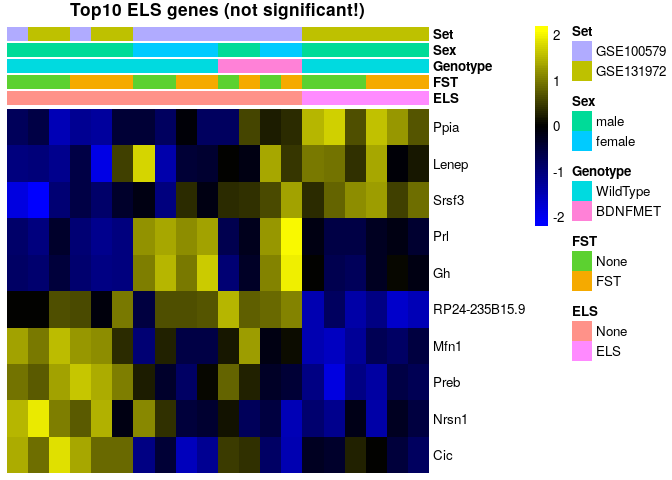
sehm(se, rownames(topTags(Results$`se$ELSELS`)), assayName = "corrected", do.scale = TRUE, anno_columns=c("ELS","FST","Genotype","Sex","Set"), main="Top10 ELS genes (not significant!)")topTags(Results$`se$ELSELS`)## Coefficient: se$ELSELS
## logFC logCPM F PValue FDR
## Lenep 9.1125460 -0.1873914 55.50044 9.109365e-06 0.1353925
## Ppia 0.4174777 8.7140180 26.71247 9.973610e-05 0.4865339
## Preb -0.3007035 6.0293637 24.57269 1.516694e-04 0.4865339
## Prl 4.9369977 3.3207763 24.23936 1.622442e-04 0.4865339
## Gh 8.1879717 3.4292305 25.17719 1.636728e-04 0.4865339
## Cic -0.4086550 5.8799801 21.90940 2.643998e-04 0.5800735
## RP24-235B15.9 -3.5726302 -1.7079165 26.29741 2.731962e-04 0.5800735
## Srsf3 0.3135256 7.3648071 20.16951 3.889850e-04 0.7015321
## Mfn1 -0.3213889 5.3104408 19.78472 4.247991e-04 0.7015321
## Nrsn1 -0.4522485 7.6124562 18.95025 5.160413e-04 0.7121992
No genes pass multiple testing correction
To futher investigate if across all samples there is any variable that interacts with acute stress we will run a series of models that incorporate an interaction term between acute stress and any of the variables. Here, we use a glmQL models in order to better correct for type I errors.
se <- kallistodata
se <- dosvacor(se, form = ~FST + Sex + Genotype + Set + ELS + FST:Sex, form0 = ~Set)
## converting counts to integer mode
## Number of significant surrogate variables is:  2
## Iteration (out of 5 ):1  2  3  4  5
#experimental design, full additive model
design <- model.matrix(~ se$SV1 + se$SV2 + se$FST + se$Sex + se$Genotype + se$Set + se$ELS + se$FST:se$Sex)

y <- DGEList(counts=assays(se)$counts)
y <- calcNormFactors(y)
y <- estimateDisp(y,design)
y <- y[filterByExpr(y, design),]

Results <- list()
fit <- glmQLFit(y,design)
for(i in colnames(design)[-1]){
  Results[[i]] <- glmQLFTest(fit, i)
}

se <- se[,order(se$Sex,se$FST)]
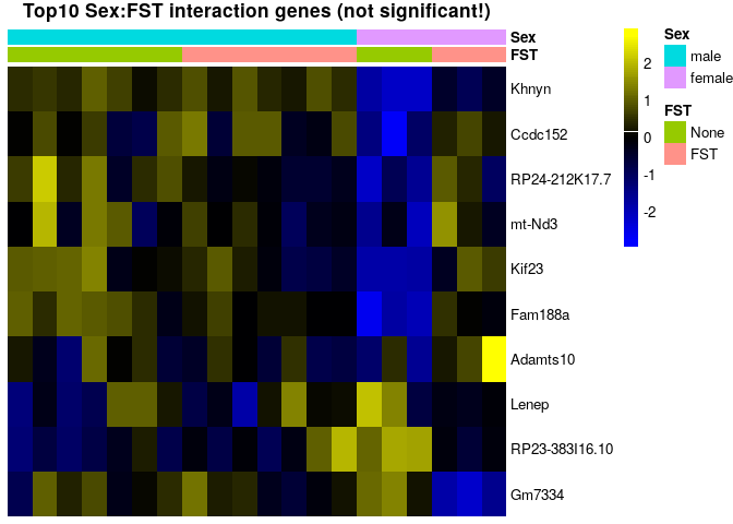
sehm(se, rownames(topTags(Results$`se$FSTFST:se$Sexfemale`)), assayName = "corrected", do.scale = TRUE, anno_columns=c("FST","Sex"), main="Top10 Sex:FST interaction genes (not significant!)")topTags(Results$`se$FSTFST:se$Sexfemale`)## Coefficient: se$FSTFST:se$Sexfemale
## logFC logCPM F PValue FDR
## Lenep -14.588936 -0.2170780 67.56013 9.647456e-06 0.1433901
## Khnyn 10.253107 -0.2975935 35.18569 5.067736e-05 0.3741113
## RP23-383I16.10 -15.955062 -2.1382336 30.56646 7.551193e-05 0.3741113
## Gm7334 -6.634741 2.1130978 24.74436 1.684480e-04 0.6259105
## Fam188a 1.381227 4.3913609 21.64146 3.162871e-04 0.8764231
## Ccdc152 3.269997 1.2683472 20.59483 3.962263e-04 0.8764231
## Kif23 4.601143 -1.7584240 19.73626 4.792222e-04 0.8764231
## RP24-212K17.7 18.211739 -2.3507779 28.34152 4.896869e-04 0.8764231
## mt-Nd3 30.108212 -1.5780609 23.12701 5.540057e-04 0.8764231
## Adamts10 28.656971 -1.7537899 24.49702 5.896677e-04 0.8764231
No genes pass multiple testing correction
se <- kallistodata
se <- dosvacor(se, form = ~FST + Sex + Genotype + Set + ELS + FST:Genotype, form0 = ~Set)
## converting counts to integer mode
## Number of significant surrogate variables is:  2
## Iteration (out of 5 ):1  2  3  4  5
#experimental design, full additive model
design <- model.matrix(~se$SV1 + se$SV2 + se$FST + se$Sex + se$Genotype + se$Set + se$ELS + se$FST:se$Genotype)

y <- DGEList(counts=assays(se)$counts)
y <- calcNormFactors(y)
y <- estimateDisp(y,design)
y <- y[filterByExpr(y, design),]


Results <- list()
fit <- glmQLFit(y,design)
for(i in colnames(design)[-1]){
  Results[[i]] <- glmQLFTest(fit, i)
}
se <- se[,order(se$Genotype,se$FST)]
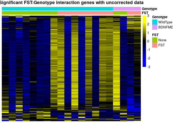
sehm(se, rownames(topTags(Results$`se$FSTFST:se$GenotypeBDNFMET`, p.value = 0.05, n = 1000)), assayName = "corrected", do.scale = TRUE, anno_columns=c("FST","Genotype"), main="Significant FST:Genotype interaction genes with corrected data")sehm(se, rownames(topTags(Results$`se$FSTFST:se$GenotypeBDNFMET`, p.value = 0.05, n = 1000)), do.scale = TRUE, anno_columns=c("FST","Genotype"), main="Significant FST:Genotype interaction genes with uncorrected data")## Using assay logcpm
topTags(Results$`se$FSTFST:se$GenotypeBDNFMET`, p.value = 0.05, n = 20)## Coefficient: se$FSTFST:se$GenotypeBDNFMET
## logFC logCPM F PValue FDR
## Sema5b 1.588439 3.100278 53.10901 2.644958e-06 0.02434796
## Setx -1.611493 6.261409 41.78315 1.061980e-05 0.02434796
## Ylpm1 -1.678628 4.838326 40.37382 1.287506e-05 0.02434796
## Nav2 -1.827796 4.907734 40.33855 1.293809e-05 0.02434796
## RP23-35L3.1 -1.501117 5.820110 39.13526 1.531347e-05 0.02434796
## Gprasp1 -2.168733 8.792082 38.60865 1.650588e-05 0.02434796
## Synm -1.206736 5.614191 36.53304 2.235000e-05 0.02434796
## Tjp1 -1.142193 5.632397 36.40322 2.278723e-05 0.02434796
## Helz -1.126191 5.241119 36.30569 2.312210e-05 0.02434796
## Lman2l 1.521352 4.930529 35.86766 2.469652e-05 0.02434796
## Arid1a -1.635858 6.382439 35.74300 2.516656e-05 0.02434796
## Nefm -1.389846 8.341769 35.55507 2.589450e-05 0.02434796
## Akap8 -1.064965 5.165599 35.11712 2.768541e-05 0.02434796
## Ryr2 -2.204308 7.528739 35.09841 2.776499e-05 0.02434796
## Lrrcc1 -1.369881 3.847630 34.83687 2.890507e-05 0.02434796
## Unc13a -1.711745 8.381426 34.48481 3.052458e-05 0.02434796
## Mdn1 -2.744802 4.535299 33.80619 3.394536e-05 0.02434796
## Dync1h1 -4.204209 9.211279 33.72648 3.437497e-05 0.02434796
## Hecw1 -1.027095 5.345130 33.70483 3.449271e-05 0.02434796
## Trio -1.280178 6.932633 33.47187 3.578909e-05 0.02434796
There are multiple genes that pass multiple testing correction. However, the data for these still looks noisy and genes that show up are highly co-expressed. The low replicate number might have impaired the ability to remove technical variability sufficiently for the Genotype:FST assessment, so the results should be interpreted with caution and more replicates would be needed.
se <- kallistodata
se <- dosvacor(se, form = ~FST + Sex + Genotype + Set + ELS + FST:ELS, form0 = ~Set)
## converting counts to integer mode
## Number of significant surrogate variables is:  2
## Iteration (out of 5 ):1  2  3  4  5
#experimental design, full additive model
design <- model.matrix(~se$SV1 + se$SV2 + se$FST + se$Sex + se$Genotype + se$Set + se$ELS + se$FST:se$ELS)

y <- DGEList(counts=assays(se)$counts)
y <- calcNormFactors(y)
y <- estimateDisp(y,design)
y <- y[filterByExpr(y, design),]

Results <- list()
fit <- glmQLFit(y,design)
for(i in colnames(design)[-1]){
  Results[[i]] <- glmQLFTest(fit, i)
}

se <- se[,order(se$ELS,se$FST)]
sehm(se, rownames(topTags(Results$`se$FSTFST:se$ELSELS`)), assayName = "corrected", do.scale = TRUE, anno_columns=c("ELS","FST"), main="Significant FST:ELS interaction genes")topTags(Results$`se$FSTFST:se$ELSELS`)## Coefficient: se$FSTFST:se$ELSELS
## logFC logCPM F PValue FDR
## Snx18 0.6895493 3.8035501 13.95823 0.002013605 1
## Parpbp 1.9365021 -0.8136012 13.92290 0.002033118 1
## Flt1 -1.8155464 0.8068678 13.90863 0.002041060 1
## Olfr133 -3.2737624 -1.6858762 12.64240 0.002910296 1
## RP24-300L5.2 -8.0118520 -1.3587377 17.54642 0.003154339 1
## Poglut1 -0.7827461 4.3601521 12.11607 0.003390993 1
## Hmga2 -1.4548305 -0.7556480 11.92536 0.003587100 1
## Hist3h2a -0.4795635 6.0135226 11.74420 0.003785455 1
## Fchsd2 0.4524863 5.0380511 11.52278 0.004045149 1
## RP24-219P17.2 4.2291993 -0.7538250 11.31275 0.004310440 1
No genes pass multiple testing correction.
Testing for interactions requires more power than simpler comparisons, and when the data does not afford sufficient power, it is preferable not to test all hypotheses, or not to give them equal weight. We therefore also tried a staged FDR calculation, which however yielded similar results.
sessionInfo()## R version 3.6.1 (2019-07-05)
## Platform: x86_64-pc-linux-gnu (64-bit)
## Running under: Ubuntu 18.04 LTS
##
## Matrix products: default
## BLAS: /usr/lib/x86_64-linux-gnu/openblas/libblas.so.3
## LAPACK: /usr/lib/x86_64-linux-gnu/libopenblasp-r0.2.20.so
##
## locale:
## [1] LC_CTYPE=C.UTF-8 LC_NUMERIC=C LC_TIME=C.UTF-8
## [4] LC_COLLATE=C.UTF-8 LC_MONETARY=C.UTF-8 LC_MESSAGES=C.UTF-8
## [7] LC_PAPER=C.UTF-8 LC_NAME=C LC_ADDRESS=C
## [10] LC_TELEPHONE=C LC_MEASUREMENT=C.UTF-8 LC_IDENTIFICATION=C
##
## attached base packages:
## [1] parallel stats4 stats graphics grDevices utils datasets
## [8] methods base
##
## other attached packages:
## [1] DESeq2_1.26.0 sva_3.34.0
## [3] genefilter_1.68.0 mgcv_1.8-31
## [5] nlme_3.1-145 SummarizedExperiment_1.16.1
## [7] DelayedArray_0.12.2 BiocParallel_1.20.1
## [9] matrixStats_0.55.0 Biobase_2.46.0
## [11] GenomicRanges_1.38.0 GenomeInfoDb_1.22.0
## [13] IRanges_2.20.2 S4Vectors_0.24.3
## [15] BiocGenerics_0.32.0 SEtools_1.2.2
## [17] edgeR_3.28.1 limma_3.42.2
##
## loaded via a namespace (and not attached):
## [1] Rtsne_0.15 colorspace_1.4-1 rjson_0.2.20
## [4] htmlTable_1.13.3 circlize_0.4.8 XVector_0.26.0
## [7] GlobalOptions_0.1.1 base64enc_0.1-3 rstudioapi_0.11
## [10] clue_0.3-57 farver_2.0.3 bit64_0.9-7
## [13] AnnotationDbi_1.48.0 codetools_0.2-16 splines_3.6.1
## [16] geneplotter_1.64.0 knitr_1.28 Formula_1.2-3
## [19] jsonlite_1.6.1 annotate_1.64.0 cluster_2.1.0
## [22] png_0.1-7 pheatmap_1.0.12 compiler_3.6.1
## [25] backports_1.1.5 assertthat_0.2.1 Matrix_1.2-18
## [28] lazyeval_0.2.2 acepack_1.4.1 htmltools_0.4.0
## [31] tools_3.6.1 gtable_0.3.0 glue_1.4.2
## [34] GenomeInfoDbData_1.2.2 dplyr_0.8.4 V8_3.0.1
## [37] Rcpp_1.0.3 vctrs_0.2.3 gdata_2.18.0
## [40] iterators_1.0.12 xfun_0.12 stringr_1.4.0
## [43] openxlsx_4.1.4 lifecycle_0.1.0 gtools_3.8.2
## [46] XML_3.99-0.3 dendextend_1.13.4 zlibbioc_1.32.0
## [49] MASS_7.3-51.5 scales_1.1.0 TSP_1.1-9
## [52] RColorBrewer_1.1-2 ComplexHeatmap_2.2.0 yaml_2.2.1
## [55] curl_4.3 memoise_1.1.0 gridExtra_2.3
## [58] ggplot2_3.2.1 rpart_4.1-15 latticeExtra_0.6-29
## [61] stringi_1.4.6 RSQLite_2.2.0 randomcoloR_1.1.0.1
## [64] gclus_1.3.2 foreach_1.4.8 checkmate_2.0.0
## [67] seriation_1.2-8 caTools_1.18.0 zip_2.0.4
## [70] shape_1.4.4 rlang_0.4.5 pkgconfig_2.0.3
## [73] bitops_1.0-6 evaluate_0.14 lattice_0.20-40
## [76] purrr_0.3.3 htmlwidgets_1.5.1 bit_1.1-15.2
## [79] tidyselect_1.0.0 magrittr_1.5 R6_2.4.1
## [82] gplots_3.0.3 Hmisc_4.3-1 DBI_1.1.0
## [85] foreign_0.8-76 pillar_1.4.3 nnet_7.3-13
## [88] survival_3.1-8 RCurl_1.98-1.1 tibble_2.1.3
## [91] crayon_1.3.4 KernSmooth_2.23-16 rmarkdown_2.1
## [94] viridis_0.5.1 jpeg_0.1-8.1 GetoptLong_0.1.8
## [97] locfit_1.5-9.4 grid_3.6.1 data.table_1.12.8
## [100] blob_1.2.1 digest_0.6.25 xtable_1.8-4
## [103] munsell_0.5.0 registry_0.5-1 viridisLite_0.3.0
