rnoaa

rnoaa is an R interface to many NOAA data sources. We don’t cover all of them, but we include many commonly used sources, and add we are always adding new sources. We focus on easy to use interfaces for getting NOAA data, and giving back data in easy to use formats downstream. We currently don’t do much in the way of plots or analysis.

Data sources in rnoaa

NOAA NCDC climate data:
- We are using the NOAA API version 2
- Docs for the NCDC API are at http://www.ncdc.noaa.gov/cdo-web/webservices/v2
- GHCN Daily data is available at http://www.ncdc.noaa.gov/oa/climate/ghcn-daily/ via FTP and HTTP
Severe weather data docs are at http://www.ncdc.noaa.gov/swdiws/
Sea ice data
NOAA buoy data
ERDDAP data
- Now in package rerddap
Tornadoes! Data from the NOAA Storm Prediction Center
HOMR - Historical Observing Metadata Repository - from NOAA NCDC
Storm data - from the International Best Track Archive for Climate Stewardship (IBTrACS)
GHCND FTP data - NOAA NCDC API has some/all (not sure really) of this data, but FTP allows to get more data more quickly
Global Ensemble Forecast System (GEFS) data
Extended Reconstructed Sea Surface Temperature (ERSST) data
Argo buoys - a global array of more than 3,000 free-drifting profiling floats that measures thetemperature and salinity of the upper 2000 m of the ocean
NOAA CO-OPS - tides and currents data
NOAA Climate Prediction Center (CPC)
Africa Rainfall Climatology version 2
Blended Sea Winds
Local Climatological Data
Storm Events Database

Help

There is a tutorial on the rOpenSci website, and there are many tutorials in the package itself, available in your R session, or on CRAN. The tutorials:

NOAA Buoy vignette
NOAA National Climatic Data Center (NCDC) vignette (examples)
NOAA NCDC attributes vignette
NOAA NCDC workflow vignette
Sea ice vignette
Severe Weather Data Inventory (SWDI) vignette
Historical Observing Metadata Repository (HOMR) vignette
Storms (IBTrACS) vignette

netcdf data

Some functions use netcdf files, including:

gefs
ersst
buoy
bsw
argo

You'll need the ncdf4 package for those functions, and those only. ncdf4 is in Suggests in this package, meaning you only need ncdf4 if you are using any of the functions listed above. You'll get an informative error telling you to install ncdf4 if you don't have it and you try to use the those functions. Installation of ncdf4 should be straightforward on any system. See https://cran.r-project.org/package=ncdf4.

NOAA NCDC Datasets

There are many NOAA NCDC datasets. All data sources work, except NEXRAD2 and NEXRAD3, for an unknown reason. This relates to ncdc_*() functions only.

Dataset	Description	Start Date	End Date	Data Coverage
GHCND	Daily Summaries	1763-01-01	2018-12-09	1.00
GSOM	Global Summary of the Month	1763-01-01	2018-11-01	1.00
GSOY	Global Summary of the Year	1763-01-01	2018-01-01	1.00
NEXRAD2	Weather Radar (Level II)	1991-06-05	2018-12-10	0.95
NEXRAD3	Weather Radar (Level III)	1994-05-20	2018-12-07	0.95
NORMAL_ANN	Normals Annual/Seasonal	2010-01-01	2010-01-01	1.00
NORMAL_DLY	Normals Daily	2010-01-01	2010-12-31	1.00
NORMAL_HLY	Normals Hourly	2010-01-01	2010-12-31	1.00
NORMAL_MLY	Normals Monthly	2010-01-01	2010-12-01	1.00
PRECIP_15	Precipitation 15 Minute	1970-05-12	2014-01-01	0.25
PRECIP_HLY	Precipitation Hourly	1900-01-01	2014-01-01	1.00

NOAA NCDC Attributes

Each NOAA dataset has a different set of attributes that you can potentially get back in your search. See http://www.ncdc.noaa.gov/cdo-web/datasets for detailed info on each dataset. We provide some information on the attributes in this package; see the vignette for attributes to find out more

NCDC Authentication

You’ll need an API key to use the NOAA NCDC functions (those starting with ncdc*()) in this package (essentially a password). Go to http://www.ncdc.noaa.gov/cdo-web/token to get one. You can’t use this package without an API key.

Once you obtain a key, there are two ways to use it.

Pass it inline with each function call (somewhat cumbersome)

ncdc(datasetid = 'PRECIP_HLY', locationid = 'ZIP:28801', datatypeid = 'HPCP', limit = 5, token =  "YOUR_TOKEN")

Alternatively, you might find it easier to set this as an option, either by adding this line to the top of a script or somewhere in your .rprofile

options(noaakey = "KEY_EMAILED_TO_YOU")

You can always store in permamently in your .Rprofile file.

Installation

GDAL

You’ll need GDAL installed first. You may want to use GDAL >= 0.9-1 since that version or later can read TopoJSON format files as well, which aren’t required here, but may be useful. Install GDAL:

OSX - From http://www.kyngchaos.com/software/frameworks
Linux - run sudo apt-get install gdal-bin reference
Windows - From http://trac.osgeo.org/osgeo4w/

Then when you install the R package rgdal (rgeos also requires GDAL), you’ll most likely need to specify where you’re gdal-config file is on your machine, as well as a few other things. I have an OSX Mavericks machine, and this works for me (there’s no binary for Mavericks, so install the source version):

install.packages("http://cran.r-project.org/src/contrib/rgdal_0.9-1.tar.gz", repos = NULL, type="source", configure.args = "--with-gdal-config=/Library/Frameworks/GDAL.framework/Versions/1.10/unix/bin/gdal-config --with-proj-include=/Library/Frameworks/PROJ.framework/unix/include --with-proj-lib=/Library/Frameworks/PROJ.framework/unix/lib")

The rest of the installation should be easy. If not, let us know.

Stable version from CRAN

install.packages("rnoaa")

or development version from GitHub

devtools::install_github("ropensci/rnoaa")

Load rnoaa

library('rnoaa')

NCDC v2 API data

Fetch list of city locations in descending order

ncdc_locs(locationcategoryid='CITY', sortfield='name', sortorder='desc')
#> $meta
#> $meta$totalCount
#> [1] 1987
#> 
#> $meta$pageCount
#> [1] 25
#> 
#> $meta$offset
#> [1] 1
#> 
#> 
#> $data
#>       mindate    maxdate                  name datacoverage            id
#> 1  1892-08-01 2018-10-31            Zwolle, NL       1.0000 CITY:NL000012
#> 2  1901-01-01 2018-12-07            Zurich, SZ       1.0000 CITY:SZ000007
#> 3  1957-07-01 2018-12-07         Zonguldak, TU       1.0000 CITY:TU000057
#> 4  1906-01-01 2018-12-07            Zinder, NG       0.9025 CITY:NG000004
#> 5  1973-01-01 2018-12-07        Ziguinchor, SG       1.0000 CITY:SG000004
#> 6  1938-01-01 2018-12-07         Zhytomyra, UP       0.9723 CITY:UP000025
#> 7  1948-03-01 2018-12-07        Zhezkazgan, KZ       0.9302 CITY:KZ000017
#> 8  1951-01-01 2018-12-07         Zhengzhou, CH       1.0000 CITY:CH000045
#> 9  1941-01-01 2018-10-31          Zaragoza, SP       1.0000 CITY:SP000021
#> 10 1936-01-01 2009-06-17      Zaporiyhzhya, UP       1.0000 CITY:UP000024
#> 11 1957-01-01 2018-12-07          Zanzibar, TZ       0.8016 CITY:TZ000019
#> 12 1973-01-01 2018-12-07            Zanjan, IR       0.9105 CITY:IR000020
#> 13 1893-01-01 2018-12-10     Zanesville, OH US       1.0000 CITY:US390029
#> 14 1912-01-01 2017-06-19             Zahle, LE       0.9819 CITY:LE000004
#> 15 1951-01-01 2018-12-07           Zahedan, IR       0.9975 CITY:IR000019
#> 16 1860-12-01 2018-12-07            Zagreb, HR       1.0000 CITY:HR000002
#> 17 1975-08-29 2018-12-07         Zacatecas, MX       0.9306 CITY:MX000036
#> 18 1947-01-01 2018-12-07 Yuzhno-Sakhalinsk, RS       1.0000 CITY:RS000081
#> 19 1893-01-01 2018-12-10           Yuma, AZ US       1.0000 CITY:US040015
#> 20 1942-02-01 2018-12-10   Yucca Valley, CA US       1.0000 CITY:US060048
#> 21 1885-01-01 2018-12-10      Yuba City, CA US       1.0000 CITY:US060047
#> 22 1998-02-01 2018-12-07            Yozgat, TU       0.9993 CITY:TU000056
#> 23 1893-01-01 2018-12-10     Youngstown, OH US       1.0000 CITY:US390028
#> 24 1894-01-01 2018-12-10           York, PA US       1.0000 CITY:US420024
#> 25 1869-01-01 2018-12-10        Yonkers, NY US       1.0000 CITY:US360031
#> 
#> attr(,"class")
#> [1] "ncdc_locs"

Get info on a station by specifying a dataset, locationtype, location, and station

ncdc_stations(datasetid='GHCND', locationid='FIPS:12017', stationid='GHCND:USC00084289')
#> $meta
#> NULL
#> 
#> $data
#>   elevation    mindate    maxdate latitude                  name
#> 1      12.2 1899-02-01 2018-12-09  28.8029 INVERNESS 3 SE, FL US
#>   datacoverage                id elevationUnit longitude
#> 1            1 GHCND:USC00084289        METERS  -82.3126
#> 
#> attr(,"class")
#> [1] "ncdc_stations"

Search for data

out <- ncdc(datasetid='NORMAL_DLY', stationid='GHCND:USW00014895', datatypeid='dly-tmax-normal', startdate = '2010-05-01', enddate = '2010-05-10')

See a data.frame

head( out$data )
#> # A tibble: 6 x 5
#>   date                datatype        station           value fl_c 
#>   <chr>               <chr>           <chr>             <int> <chr>
#> 1 2010-05-01T00:00:00 DLY-TMAX-NORMAL GHCND:USW00014895   652 S    
#> 2 2010-05-02T00:00:00 DLY-TMAX-NORMAL GHCND:USW00014895   655 S    
#> 3 2010-05-03T00:00:00 DLY-TMAX-NORMAL GHCND:USW00014895   658 S    
#> 4 2010-05-04T00:00:00 DLY-TMAX-NORMAL GHCND:USW00014895   661 S    
#> 5 2010-05-05T00:00:00 DLY-TMAX-NORMAL GHCND:USW00014895   663 S    
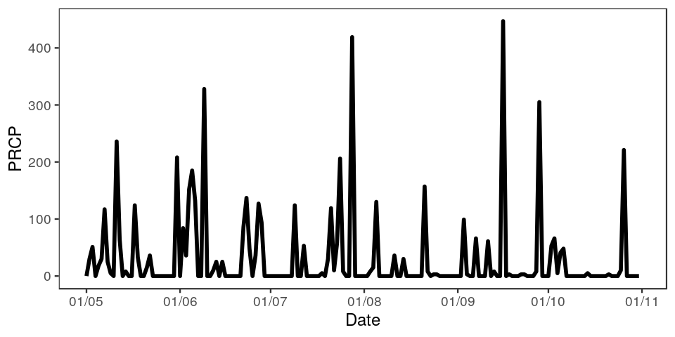
#> 6 2010-05-06T00:00:00 DLY-TMAX-NORMAL GHCND:USW00014895   666 S

Plot data, super simple, but it’s a start

out <- ncdc(datasetid='GHCND', stationid='GHCND:USW00014895', datatypeid='PRCP', startdate = '2010-05-01', enddate = '2010-10-31', limit=500)
ncdc_plot(out, breaks="1 month", dateformat="%d/%m")

More plotting

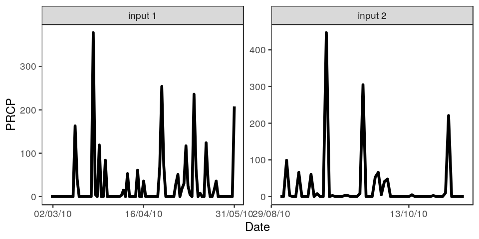
You can pass many outputs from calls to the noaa function in to the ncdc_plot function.

out1 <- ncdc(datasetid='GHCND', stationid='GHCND:USW00014895', datatypeid='PRCP', startdate = '2010-03-01', enddate = '2010-05-31', limit=500)
out2 <- ncdc(datasetid='GHCND', stationid='GHCND:USW00014895', datatypeid='PRCP', startdate = '2010-09-01', enddate = '2010-10-31', limit=500)
ncdc_plot(out1, out2, breaks="45 days")

Get table of all datasets

ncdc_datasets()
#> $meta
#> $meta$offset
#> [1] 1
#> 
#> $meta$count
#> [1] 11
#> 
#> $meta$limit
#> [1] 25
#> 
#> 
#> $data
#>                     uid    mindate    maxdate                        name
#> 1  gov.noaa.ncdc:C00861 1763-01-01 2018-12-09             Daily Summaries
#> 2  gov.noaa.ncdc:C00946 1763-01-01 2018-11-01 Global Summary of the Month
#> 3  gov.noaa.ncdc:C00947 1763-01-01 2018-01-01  Global Summary of the Year
#> 4  gov.noaa.ncdc:C00345 1991-06-05 2018-12-10    Weather Radar (Level II)
#> 5  gov.noaa.ncdc:C00708 1994-05-20 2018-12-07   Weather Radar (Level III)
#> 6  gov.noaa.ncdc:C00821 2010-01-01 2010-01-01     Normals Annual/Seasonal
#> 7  gov.noaa.ncdc:C00823 2010-01-01 2010-12-31               Normals Daily
#> 8  gov.noaa.ncdc:C00824 2010-01-01 2010-12-31              Normals Hourly
#> 9  gov.noaa.ncdc:C00822 2010-01-01 2010-12-01             Normals Monthly
#> 10 gov.noaa.ncdc:C00505 1970-05-12 2014-01-01     Precipitation 15 Minute
#> 11 gov.noaa.ncdc:C00313 1900-01-01 2014-01-01        Precipitation Hourly
#>    datacoverage         id
#> 1          1.00      GHCND
#> 2          1.00       GSOM
#> 3          1.00       GSOY
#> 4          0.95    NEXRAD2
#> 5          0.95    NEXRAD3
#> 6          1.00 NORMAL_ANN
#> 7          1.00 NORMAL_DLY
#> 8          1.00 NORMAL_HLY
#> 9          1.00 NORMAL_MLY
#> 10         0.25  PRECIP_15
#> 11         1.00 PRECIP_HLY
#> 
#> attr(,"class")
#> [1] "ncdc_datasets"

Get data category data and metadata

ncdc_datacats(locationid = 'CITY:US390029')
#> $meta
#> $meta$totalCount
#> [1] 38
#> 
#> $meta$pageCount
#> [1] 25
#> 
#> $meta$offset
#> [1] 1
#> 
#> 
#> $data
#>                     name            id
#> 1    Annual Agricultural        ANNAGR
#> 2     Annual Degree Days         ANNDD
#> 3   Annual Precipitation       ANNPRCP
#> 4     Annual Temperature       ANNTEMP
#> 5    Autumn Agricultural         AUAGR
#> 6     Autumn Degree Days          AUDD
#> 7   Autumn Precipitation        AUPRCP
#> 8     Autumn Temperature        AUTEMP
#> 9               Computed          COMP
#> 10 Computed Agricultural       COMPAGR
#> 11           Degree Days            DD
#> 12      Dual-Pol Moments DUALPOLMOMENT
#> 13             Echo Tops       ECHOTOP
#> 14      Hydrometeor Type   HYDROMETEOR
#> 15            Miscellany          MISC
#> 16                 Other         OTHER
#> 17               Overlay       OVERLAY
#> 18         Precipitation          PRCP
#> 19          Reflectivity  REFLECTIVITY
#> 20    Sky cover & clouds           SKY
#> 21   Spring Agricultural         SPAGR
#> 22    Spring Degree Days          SPDD
#> 23  Spring Precipitation        SPPRCP
#> 24    Spring Temperature        SPTEMP
#> 25   Summer Agricultural         SUAGR
#> 
#> attr(,"class")
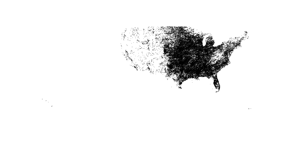
#> [1] "ncdc_datacats"

Tornado data

The function tornadoes() simply gets all the data. So the call takes a while, but once done, is fun to play with.

shp <- tornadoes()
#> OGR data source with driver: ESRI Shapefile 
#> Source: "/home/jose/.cache/rnoaa/tornadoes/torn", layer: "torn"
#> with 62520 features
#> It has 21 fields
library('sp')
plot(shp)

HOMR metadata

In this example, search for metadata for a single station ID

homr(qid = 'COOP:046742')
#> $`20002078`
#> $`20002078`$id
#> [1] "20002078"
#> 
#> $`20002078`$head
#>                  preferredName latitude_dec longitude_dec precision
#> 1 PASO ROBLES MUNICIPAL AP, CA      35.6697     -120.6283   DDddddd
#>             por.beginDate por.endDate
#> 1 1949-10-05T00:00:00.000     Present
#> 
#> $`20002078`$namez
#>                         name  nameType
#> 1   PASO ROBLES MUNICIPAL AP      COOP
#> 2   PASO ROBLES MUNICIPAL AP PRINCIPAL
#> 3 PASO ROBLES MUNICIPAL ARPT       PUB
#> 
#> $`20002078`$identifiers
#>      idType          id
#> 1     GHCND USW00093209
#> 2   GHCNMLT USW00093209
...

Storm data

Get storm data for the year 2010

storm_data(year = 2010)
#> # A tibble: 2,787 x 200
#>    serial_num season   num basin sub_basin name  iso_time nature latitude
#>    <chr>       <int> <int> <chr> <chr>     <chr> <chr>    <chr>     <dbl>
#>  1 2009317S1…   2010     1 " SI" " MM"     ANJA  2009-11… " TS"      -9.5
#>  2 2009317S1…   2010     1 " SI" " MM"     ANJA  2009-11… " TS"     -10.2
#>  3 2009317S1…   2010     1 " SI" " MM"     ANJA  2009-11… " TS"     -11.1
#>  4 2009317S1…   2010     1 " SI" " MM"     ANJA  2009-11… " TS"     -11.9
#>  5 2009317S1…   2010     1 " SI" " MM"     ANJA  2009-11… " TS"     -12.5
#>  6 2009317S1…   2010     1 " SI" " MM"     ANJA  2009-11… " TS"     -12.8
#>  7 2009317S1…   2010     1 " SI" " MM"     ANJA  2009-11… " TS"     -12.9
#>  8 2009317S1…   2010     1 " SI" " MM"     ANJA  2009-11… " TS"     -12.9
#>  9 2009317S1…   2010     1 " SI" " MM"     ANJA  2009-11… " TS"     -13  
#> 10 2009317S1…   2010     1 " SI" " MM"     ANJA  2009-11… " TS"     -13.1
#> # ... with 2,777 more rows, and 191 more variables: longitude <dbl>,
#> #   wind.wmo. <dbl>, pres.wmo. <dbl>, center <chr>,
#> #   wind.wmo..percentile <dbl>, pres.wmo..percentile <dbl>,
#> #   track_type <chr>, latitude_for_mapping <dbl>,
#> #   longitude_for_mapping <dbl>, current.basin <chr>,
#> #   hurdat_atl_lat <dbl>, hurdat_atl_lon <dbl>, hurdat_atl_grade <dbl>,
#> #   hurdat_atl_wind <dbl>, hurdat_atl_pres <dbl>, td9636_lat <dbl>,
...

GEFS data

Get forecast for a certain variable.

res <- gefs("Total_precipitation_surface_6_Hour_Accumulation_ens", lat = 46.28125, lon = -116.2188)
head(res$data)
#>   Total_precipitation_surface_6_Hour_Accumulation_ens lon lat ens time2
#> 1                                                0.45 244  46   0     6
#> 2                                                0.40 244  46   1     6
#> 3                                                0.18 244  46   2     6
#> 4                                                0.30 244  46   3     6
#> 5                                                0.60 244  46   4     6
#> 6                                                0.13 244  46   5     6

Argo buoys data

There are a suite of functions for Argo data, a few egs:

# Spatial search - by bounding box
argo_search("coord", box = c(-40, 35, 3, 2))

# Time based search
argo_search("coord", yearmin = 2007, yearmax = 2009)

# Data quality based search
argo_search("coord", pres_qc = "A", temp_qc = "A")

# Search on partial float id number
argo_qwmo(qwmo = 49)

# Get data
argo(dac = "meds", id = 4900881, cycle = 127, dtype = "D")

CO-OPS data

Get daily mean water level data at Fairport, OH (9063053)

coops_search(station_name = 9063053, begin_date = 20150927, end_date = 20150928,
             product = "daily_mean", datum = "stnd", time_zone = "lst")
#> $metadata
#> $metadata$id
#> [1] "9063053"
#> 
#> $metadata$name
#> [1] "Fairport"
#> 
#> $metadata$lat
#> [1] "41.7597"
#> 
#> $metadata$lon
#> [1] "-81.2811"
#> 
#> 
#> $data
#>            t       v   f
#> 1 2015-09-27 174.430 0,0
#> 2 2015-09-28 174.422 0,0

HONG1992/rnoaa