Predicting Bank Client's Certificate of Deposit Purchase using Scikit Learn and XGBoost for imbalance dataset

This Code Pattern will guide you through how to use XGBoost, Scikit Learn and Python in IBM Watson Studio. The goal is to use a Jupyter notebook and data from the UCI repository for Bank Marketing Data to predict if a client will purchase a Certificate of Deposit (CD) from a banking institution.

Class imbalance is a common problem in data science, where the number of positive samples are significantly less than the number of negative samples. As data scientists, one would like to solve this problem and create a classifier with good performance. XGBoost (Extreme Gradient Boosting Decision Tree) is very common tool for creating the Machine Learning Models for classification and regression. However, there are various tricks and techniques for creating good classification models using XGBoost for imbalanced data-sets that is non-trivial and the reason for developing this Code Pattern.

In this Code Pattern, we will illustrate how the Machine Learning classification is performed using XGBoost, which is usually a better choice compared to logistic regression and other techniques. We will use a real life data set which is highly imbalanced (i.e the number of positive sample is much less than the number of negative samples).

This Code Pattern will walk the user through the following conceptual steps:

Data Set Description.
Exploratory Analysis to understand the data.
Use various preprocessing to clean and prepare the data.
Use naive XGBoost to run the classification.
- Use cross validation to get the model.
- Plot, precision recall curve and ROC curve.
We will then tune it and use weighted positive samples to improve classification performance.
We will also talk about the following advanced techniques.
- Oversampling of majority class and Undersampling of minority class.
- SMOTE algorithms.

Notebooks

predict_bank_cd_subs_by_xgboost_clf_for_imbalance_dataset.ipynb: The main notebook we'll be using in this exercise.

Flow

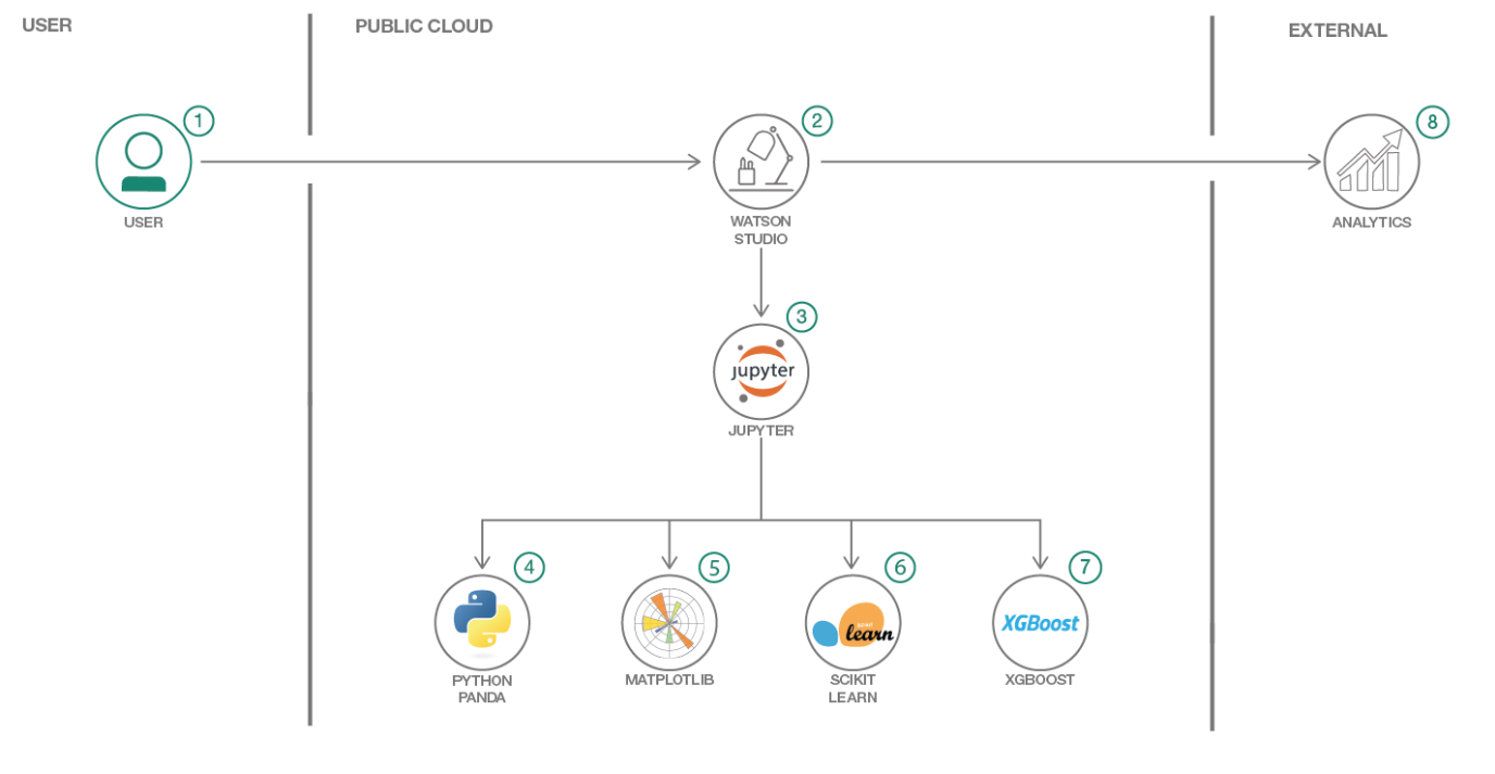
Log into IBM Watson Studio service.
Upload the data as a data asset into Watson Studio.
Start a notebook in Watson Studio and input the data asset previously created.
Pandas are used to read the data file into a dataframe for initial data exploration.
Use Matplotlib and it's higher level package seaborn for creating various visualizations.
Use Scikit Learn to create our ML pipeline to prep our data to be fed into XGBoost.
Use XGBoost to create and train our ML model.
Evaluate their predictive performance.

Included components

IBM Watson Studio: Analyze data using RStudio, Jupyter, and Python in a configured, collaborative environment that includes IBM value-adds, such as managed Spark.
Jupyter Notebook: An open source web application that allows you to create and share documents that contain live code, equations, visualizations, and explanatory text.

Featured technologies

Data Science: Systems and scientific methods to analyze structured and unstructured data in order to extract knowledge and insights.
Python: Python is a programming language that lets you work more quickly and integrate your systems more effectively.
XGBoost: Extreme Gradient Boosting is decision tree based tools for creating ML model.
Scikit Learn: A Python library for providing efficient tools for data mining and machine learning.
Pandas: A Python library providing high-performance, easy-to-use data structures.
Matplotlib: A Python library integrating matplot for visualization.
SeaBorn: Another higher level Python library for visualization.

Steps

This Code Pattern consists of following activities:

Run a Jupyter notebook in the IBM Watson Studio.
Explore, Analyze and Predict CD Subscription for Bank Client.

Run a Jupyter notebook in the IBM Watson Studio

Create a new Watson Studio project
Create the notebook
Upload data
Run the notebook
Save and Share

1. Create a new Watson Studio project

Log into IBM's Watson Studio. Once in, you'll land on the dashboard.
Create a new project by clicking + New project and choosing Data Science:
Enter a name for the project name and click Create.
NOTE: By creating a project in Watson Studio a free tier Object Storage service and Watson Machine Learning service will be created in your IBM Cloud account. Select the Free storage type to avoid fees.
Upon a successful project creation, you are taken to a dashboard view of your project. Take note of the Assets and Settings tabs, we'll be using them to associate our project with any external assets (datasets and notebooks) and any IBM cloud services.

2. Create the Notebook

From the new project Overview panel, click + Add to project on the top right and choose the Notebook asset type.

Fill in the following information:
- Select the From URL tab. [1]
- Enter a Name for the notebook and optionally a description. [2]
- Under Notebook URL provide the following url: https://github.com/IBM/xgboost-financial-predictions/blob/master/notebooks/predict_bank_cd_subs_by_xgboost_clf_for_imbalance_dataset.ipynb [3]
- For Runtime select the Python 3.5 option. [4]
Click the Create button.
TIP: Once successfully imported, the notebook should appear in the Notebooks section of the Assets tab.

3. Upload data

This project uses the dataset in data/bank.csv. We need to load this asset to our project.
From the new project Overview panel, click + Add to project on the top right and choose the Data asset type.
A panel on the right of the screen will appear to assit you in uploading data. Follow the numbered steps in the image below.
- Ensure you're on the Load tab. [1]
- Click on the browse option. From your machine, browse to the location of the bank.csv file in this repository, and upload it. [not numbered]
- Once uploaded, go to the Files tab. [2]
- Ensure the bank.csv appears. [3]

4. Run the notebook

Click the (►) Run button to start stepping through the notebook.
Stop at the Data Exploration section.
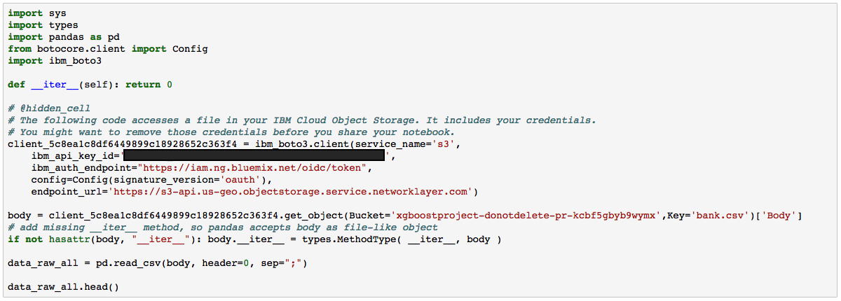
To load the data asset into the notebook, you first need to clear out the cell of all code except for the last two lines (i.e. keep the last two lines that reference data_row_all). Then place the cursor at the top of the cell above the 2 remaining lines of code.
Click on the 1001 data icon in the top right. The bank.csv data file should show up.
Click on it and select Insert Pandas Data Frame. Once you do that, a whole bunch of code will show up in your cell.
Remove the last two lines of the inserted code. These lines start with df_data_1 and will cause errors if left in.
When complete, this is what your cell should look like:

5. Save and Share

How to save your work:

Under the File menu, there are several ways to save your notebook:

Save will simply save the current state of your notebook, without any version information.
Save Version will save your current state of your notebook with a version tag that contains a date and time stamp. Up to 10 versions of your notebook can be saved, each one retrievable by selecting the Revert To Version menu item.

How to share your work:

You can share your notebook by selecting the Share button located in the top right section of your notebook panel. The end result of this action will be a URL link that will display a “read-only” version of your notebook. You have several options to specify exactly what you want shared from your notebook:

Only text and output: will remove all code cells from the notebook view.
All content excluding sensitive code cells: will remove any code cells that contain a sensitive tag. For example, # @hidden_cell is used to protect your credentials from being shared.
All content, including code: displays the notebook as is.
A variety of download as options are also available in the menu.

Explore, Analyze and Predict CD Subscription for Bank Client

1. Explore the dataset

The imbalanced dataset is from Portuguese banking institutions, and is based on phone calls to bank clients regarding the purchase of financial products offered by the bank (ie. Certificates of Deposit).

2. Prepare the data

For this section we will mostly use Python based libraries such as XGBoost, Scikit-learn, Matplotlib, SeaBorn, and Pandas.

3. Visual Data Exploration to understand the data using Seaborn and Matplotlib

Data scientists typically perform data exploration to gain better insight into data. Here we will explore inputs for distribution, correlation and outliers, and outputs to note any class imbalance issues.

4. Create Scikit learn ML Pipelines for Data Processing

Split the data into train and test sets.
Create an ML pipeline for data preparation.

In typical machine learning applications, an ML pipeline is created so that all the steps that are done on a training data set can be easily applied to the test set.

5. Model Training and evaluation

Model Training is a iterative process and we will do several iterations to improve our model performance.

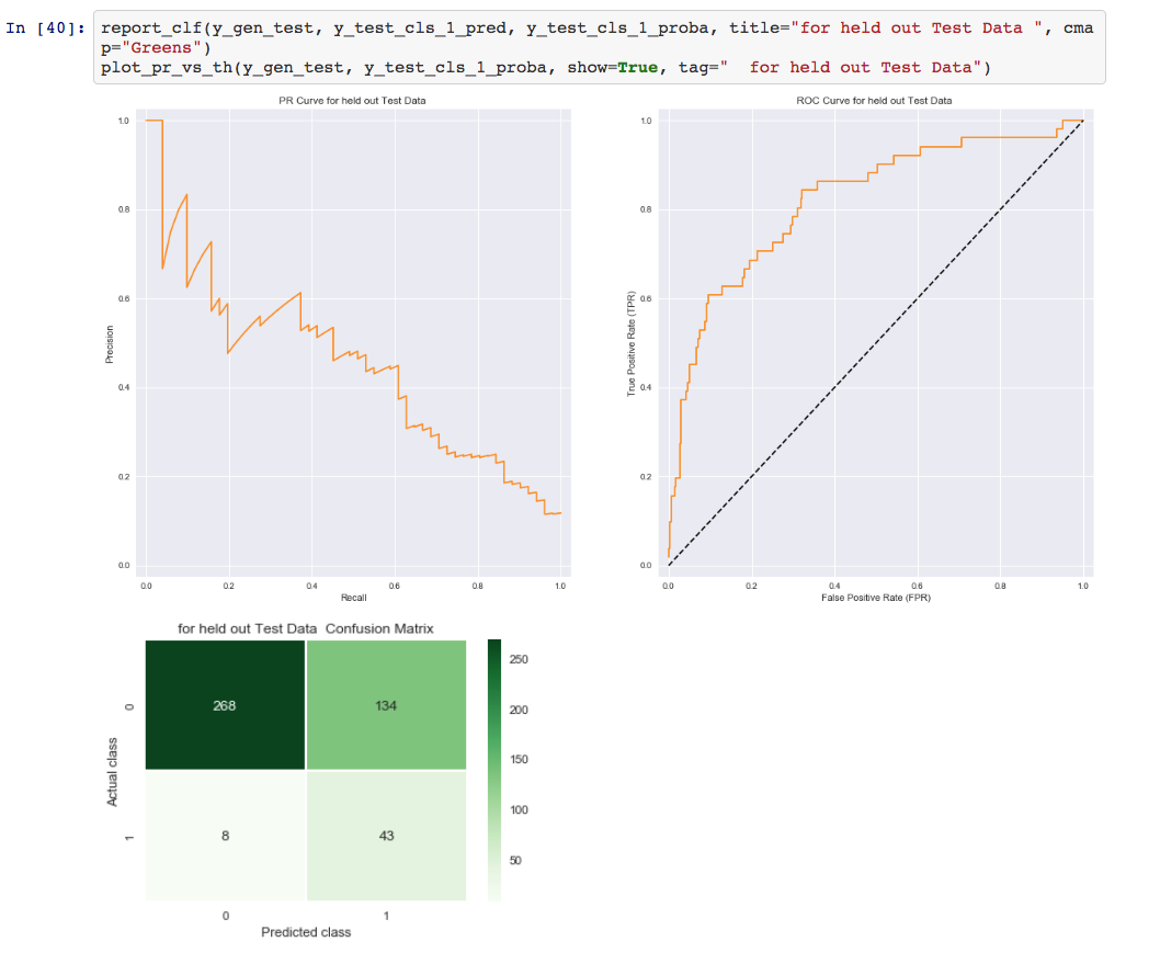
Using XGBoost as our tool of choice, we will highlight classification performance metrics such as ROC curve, Precision-Recall curve, and Confusion Matrix.

We then offer multiple strategies to improve our classifier performance.

6. Inference Discussion (Generalization and Prediction)

In many ML training applications, there is the risk that the model won't generalize enough for unknown data. To mitigate this, it is recommended that data scientists do generalization error testing. This involves running cross validated models to predict on held-out data, to see it's performance on test data. But it's important that we don't look at held-out data or use it in training because this can make our model training biased and result in a large generalization error.

Sample Output

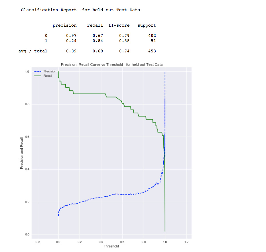
The following screen-shots show that we set the weight on the positive sample to be 1000 and the feature selection threshold to be 0.008. In the third attempt running this tuned classifier, we find that our recall for an imbalanced positive sample has improved to 0.84 on the test data.

Awesome job following along! Now go try and take this further or apply it to a different use case!

Learn more

Data Analytics Code Patterns: Enjoyed this Code Pattern? Check out our other Data Analytics Code Patterns
AI and Data Code Pattern Playlist: Bookmark our playlist with all of our Code Pattern videos
Watson Studio: Master the art of data science with IBM's Watson Studio

License

This code pattern is licensed under the Apache License, Version 2. Separate third-party code objects invoked within this code pattern are licensed by their respective providers pursuant to their own separate licenses. Contributions are subject to the Developer Certificate of Origin, Version 1.1 and the Apache License, Version 2.

Apache License FAQ

IBM/xgboost-financial-predictions