This package provides utilities for eddy covariance data handling, quality checking (similar to Mauder et al., 2013), processing, summarising and plotting. It aims to standardise the automated quality checking and make data processing reproducible.
-
Install devtools package if not available yet.
install.packages("devtools") -
Install openeddy
devtools::install_github("lsigut/openeddy")
An extended example describing the intended eddy covariance data processing workflow is available at:
https://github.com/lsigut/EC_workflow
Demonstration of selected generally applicable openeddy functions.
library(openeddy)
#>
#> Attaching package: 'openeddy'
#> The following objects are masked from 'package:base':
#>
#>     units, units<-
library(REddyProc)
library(ggplot2)
Example data from REddyProc package do not include statistics extracted from raw data or quality control (QC) flags. Notice that units are included.
data(Example_DETha98)
str(Example_DETha98[1:4])
#> 'data.frame':    17520 obs. of  4 variables:
#>  $ Year: int  1998 1998 1998 1998 1998 1998 1998 1998 1998 1998 ...
#>   ..- attr(*, "varnames")= chr "Year"
#>   ..- attr(*, "units")= chr "-"
#>  $ DoY : int  1 1 1 1 1 1 1 1 1 1 ...
#>   ..- attr(*, "varnames")= chr "DoY"
#>   ..- attr(*, "units")= chr "-"
#>  $ Hour: num  0.5 1 1.5 2 2.5 3 3.5 4 4.5 5 ...
#>   ..- attr(*, "varnames")= chr "Hour"
#>   ..- attr(*, "units")= chr "-"
#>  $ NEE : num  -1.21 1.72 NA NA 2.55 NA NA NA 4.11 NA ...
#>   ..- attr(*, "varnames")= chr "NEE"
#>   ..- attr(*, "units")= chr "umolm-2s-1"
DETha98 <- fConvertTimeToPosix(Example_DETha98, 'YDH',
                               Year = 'Year', Day = 'DoY', Hour = 'Hour')
#> Converted time format 'YDH' to POSIX with column name 'DateTime'.
Certain variable names are expected by openeddy, thus DETha98 variable names need to be renamed. Net ecosystem exchange (NEE) is already filtered based on QC information (qc_NEE) that is not included. Though flag 2 values can be recreated, respective NEE values are missing and flag 1 cannot be resolved.
rename <- names(DETha98) %in% c("DateTime", "Rg")
names(DETha98)[rename] <- c("timestamp", "GR")
DETha98$qc_NEE <- ifelse(is.na(DETha98$NEE), NA, 0)
Application of three general filters is presented.
- Low covariance between vertical wind component and CO2 concentration ((CO2)) can be caused by frozen ultrasonic anemometer or problems with (CO2) measurements. Such cases are flagged and saved to qc_NEE_lowcov.
- Runs with repeating values are a sign of malfunctioning equipment (qc_NEE_runs).
- Spikes in low frequency data cause problems during gap-filling and should be excluded. Since DETha98 was already quality checked, the amount of detected spikes is limited. In order to correctly evaluate spikes, preliminary QC (qc_NEE_prelim) that combines available QC tests or filters should be produced and used in
despikeLF.
DETha98$qc_NEE_lowcov <-
  apply_thr(DETha98$NEE, c(-0.01, 0.01), "qc_NEE_lowcov", "between")
table(DETha98$qc_NEE_lowcov)
#>
#>     0     2
#> 11251    12
DETha98$qc_NEE_runs <- flag_runs(DETha98$NEE, "qc_NEE_runs")
table(DETha98$qc_NEE_runs)
#>
#>     0     2
#> 11064   199
DETha98$qc_NEE_prelim <-
  combn_QC(DETha98,
           c("qc_NEE", "qc_NEE_lowcov", "qc_NEE_runs"),
           "qc_NEE_prelim", additive = FALSE, na.as = NA)
DETha98$qc_NEE_despikeLF <-
  despikeLF(DETha98, "NEE", "qc_NEE_prelim", "qc_NEE_despikeLF",
            light = NULL)
#> iter 1: 25
#> iter 2: 1
#> iter 3: 0
#> Further iterations omitted
table(DETha98$qc_NEE_despikeLF)
#>
#>     0     2
#> 11024    26
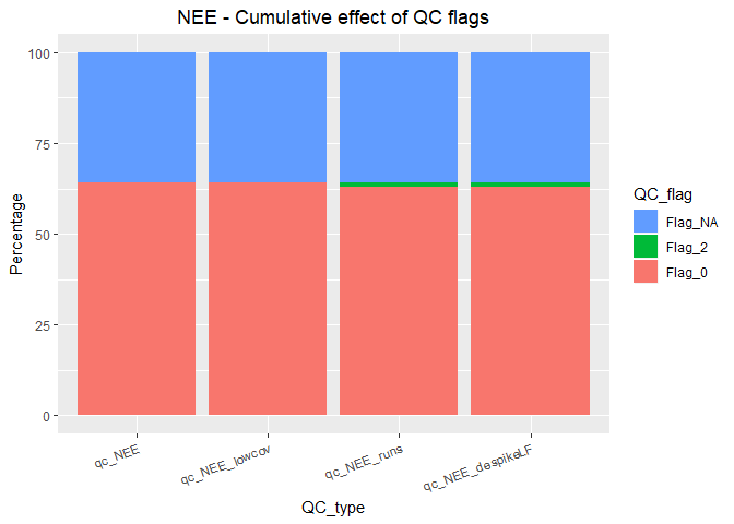
The QC results can be summarized in tabular or graphical form using summary_QC. It is possible to summarize each filter independently or summarize the cummulative effect of applied filters. Note that the fraction of flagged records in this example is negligible as DETha98 dataset was already quality checked.
summary_QC(DETha98,
           c("qc_NEE", "qc_NEE_lowcov", "qc_NEE_runs", "qc_NEE_despikeLF"),
           na.as = c(NA, NA, NA, 0))
#>                   QC_flag
#> QC_type               0    2 <NA>
#>   qc_NEE           64.3  0.0 35.7
#>   qc_NEE_lowcov    64.2  0.1 35.7
#>   qc_NEE_runs      63.2  1.1 35.7
#>   qc_NEE_despikeLF 99.9  0.1  0.0
summary_QC(DETha98,
           c("qc_NEE", "qc_NEE_lowcov", "qc_NEE_runs", "qc_NEE_despikeLF"),
           na.as = c(NA, NA, NA, 0), cumul = TRUE, plot = TRUE, flux = "NEE")
Although individual QC columns should be stored as they are useful to distinguish the reason why certain records were excluded, only the combined QC column (qc_NEE_composite) is usually used in further data processing and analysis.
DETha98$qc_NEE_composite <-
  combn_QC(DETha98,
           c("qc_NEE", "qc_NEE_lowcov", "qc_NEE_runs", "qc_NEE_despikeLF"),
           "qc_NEE_composite", additive = FALSE, na.as = c(NA, NA, NA, 0))
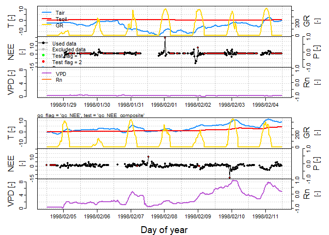
Function plot_eddy is useful for visualization of the whole dataset including flux values, its respective QC flags and the most important micrometeorological parameters in monthly and weekly time resolution. Only a two week subset is presented here to limit the extent of output.
DETha98[, c("P", "PAR", "Rn")] <- NA
(varnames <- varnames(DETha98))
#>  [1] "DateTime"         "Year"             "DoY"
#>  [4] "Hour"             "NEE"              "LE"
#>  [7] "H"                "Rg"               "Tair"
#> [10] "Tsoil"            "rH"               "VPD"
#> [13] "Ustar"            "-"                "qc_NEE_lowcov"
#> [16] "qc_NEE_runs"      "qc_NEE_prelim"    "qc_NEE_despikeLF"
#> [19] "qc_NEE_composite" "-"                "-"
#> [22] "-"
(units <- openeddy::units(DETha98))
#>  [1] "POSIXDate Time" "-"              "-"              "-"
#>  [5] "umolm-2s-1"     "Wm-2"           "Wm-2"           "Wm-2"
#>  [9] "degC"           "degC"           "%"              "hPa"
#> [13] "ms-1"           "-"              "-"              "-"
#> [17] "-"              "-"              "-"              "-"
#> [21] "-"              "-"
sub <- DETha98$DoY >= 29 & DETha98$DoY < 43
DETha98_sub <- DETha98[sub, ]
openeddy::units(DETha98) <- units
plot_eddy(DETha98_sub, "NEE", "qc_NEE", "qc_NEE_composite", skip = "monthly",
          light = "GR")
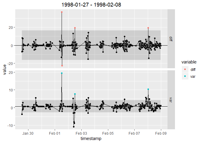
In addition to actual despiking, despikeLF can be used also for visualization of the internally computed double-differenced time series in order to inspect selected 13 days blocks. See section Plotting in despikeLF help file for further description.
despikeLF_plots <-
  despikeLF(DETha98, "NEE", "qc_NEE_prelim", "qc_NEE_despikeLF",
            light = NULL, plot = TRUE)$plots
#> iter 1: 25
#> iter 2: 1
#> iter 3: 0
#> Further iterations omitted
despikeLF_plots$`iter 1`$all$`1998-01-27 - 1998-02-08`Publication describing openeddy is not yet available. When describing the proposed quality control scheme, please refer to it as similar to:
Mauder, M., Cuntz, M., Drüe, C., Graf, A., Rebmann, C., Schmid, H.P., Schmidt, M., Steinbrecher, R., 2013. A strategy for quality and uncertainty assessment of long-term eddy-covariance measurements. Agric. For. Meteorol. 169, 122-135, https://doi.org/10.1016/j.agrformet.2012.09.006


