98,9 % Validation Accuracy - CarND-Traffic-Sign-Classifier-Project
In this project, I use what I've learned about deep neural networks and convolutional neural networks in Udacity's Traffic sign classification project which is part of their Self-driving Car Nano Degree. Specifically, train a model to classify traffic signs from the German Traffic Sign Dataset.
Build a Traffic Sign Recognition Project
The goals / steps of this project are the following:
- Load the data set (see below for links to the project data set)
- Explore, summarize and visualize the data set
- Normalize and augment the dataset
- Design, train and test a model architecture
- Use the model to make predictions on new images
- Analyze the softmax probabilities of the new images
- Summarize the results with a written report
Writeup / README
1. Provide a Writeup / README that includes all the rubric points and how you addressed each one. You can submit your writeup as markdown or pdf. You can use this template as a guide for writing the report. The submission includes the project code.
I achieved a validation set accuracy of 98,9 % and test set accuracy of 97,9 % with this project code (.ipynb-file), html can be found here! In this Notebook I set the augmentation minimum to 200 for time saving reason, but you can comment out the manual overide of the variable mean_no_of_samples = 200 or set it to a value of desire. You could also load the pre normalized and augmented data, more of this topic below.
Data Set Summary & Exploration
1. Provide a basic summary of the data set. In the code, the analysis should be done using python, numpy and/or pandas methods rather than hardcoding results manually.
I used the pandas library to calculate summary statistics of the traffic signs data set:
- The size of the training set is: 34799 images
- The size of the validation set is: 4410 images
- The size of the test set is: 12630 images
- The shape of a traffic sign image is: 32 pixel * 32 pixel * 3 colorchannel
- The number of unique classes/labels in the data set is: 43
2. Include an exploratory visualization of the dataset.
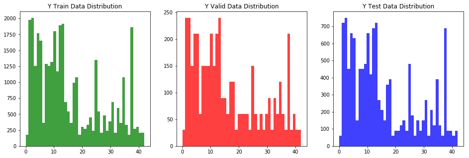
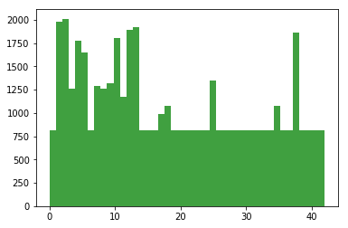
First there is a bar chart showing how the classes are distributed, as you can see some classes are very underrepresented. This can lead to problems, because then the ConvNet will be biased towards classes with a lot of images. If I give a hundred yield signs, a stop sign, then two hundred more yield signs, it is pretty predictable in which direction the CNN will lean.
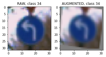
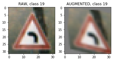
Futhermore here are some exemplary representation of random classes and images (title is class) :
Design and Test a Model Architecture
1. Describe how you preprocessed the image data. What techniques were chosen and why did you choose these techniques? Consider including images showing the output of each preprocessing technique. Pre-processing refers to techniques such as converting to grayscale, normalization, etc. (OPTIONAL: As described in the "Stand Out Suggestions" part of the rubric, if you generated additional data for training, describe why you decided to generate additional data, how you generated the data, and provide example images of the additional data. Then describe the characteristics of the augmented training set like number of images in the set, number of images for each class, etc.)
-
I didn't convert to grayscale because some testing showed that the CNN learned better with the additionally color information, which is understandable.
-
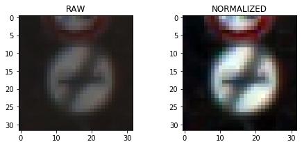
First I normalized all images to a scale of -1, 1 by getting the maximum and minimum of each color channel of each image, calculating the range with the Max&Mins and then apply following formula :
image[:,:, color] = (image[:,:,color] - (val_range/2 + min_val)) / (val_range/2)After normalization I'm getting close to 0-centered data, which is essential for good machine earning.
Mean of raw data: 82.677589037Mean of normalized data: -0.305579028335Example:
-
As described in Data Set Summary & Exploration underrepresented classes can lead to problems. Another topic is invariance: To make the CNN robust it has to learn all kinds of rotation, scaling, lighting, etc. , to achieve this invariance I decided to augment more data. These following techniques were used:
- random Colorshift: Each colorchannel will be multiplied by a random factor between the low limit (which you can set) and 1
- random Warp: The image is randomly warped to simulated different viewing angles. Also adjustable
- random Zoom: The image is randomly zoomed in an adjustable range
- random Rotate: The image is randomly rotated in an adjustable degree range
- random move: The image is randomly moved pixelwise by a random value in x and a seperate random value in y direction
- return this images as an augmented image
- loop through each class until number of images in class >= mean number of images over all classes
Finally I used the following ranges for augmentation:
aug_ranges: [0.12, 0.06, 7, 2, 4]- 0.12 => multiply each color randomly by a factor in range of 88 - 100%
- 0.06 => zoom randomly by a factor in range of 93 - 107 %
- 7 => rotate randomly in range of -9, 9 degree
- 2 => move randomly in range of -3, 3 pixel
- 4 => warpfactor
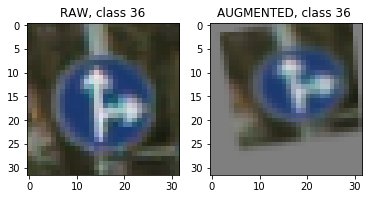
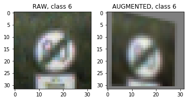
I wrote the function augmen_img, which takes an image and the aug_ranges as input and generates a new image. After a lot of trial&error I decided to use getAffineTransform & warpAffine from the library cv2 for 3 of the 5 operations, this resulted in increased generation time, but the results are very good (no pixel artefacts, etc.). To save time I concatenate the additional images to X_train and y_train and dumped it as a new p.file. New dimensions are: X_train shape: (46740, 32, 32, 3). The .p-file can be found here(augmented to minimum of 810 images in each class) and here (minimum 400 images)
Here are some examples of an original image and an augmented image:
Distribution after augmentation, every class has atleast (mean number of samples in X_train =) 810 images:
2. Describe what your final model architecture looks like including model type, layers, layer sizes, connectivity, etc.) Consider including a diagram and/or table describing the final model.
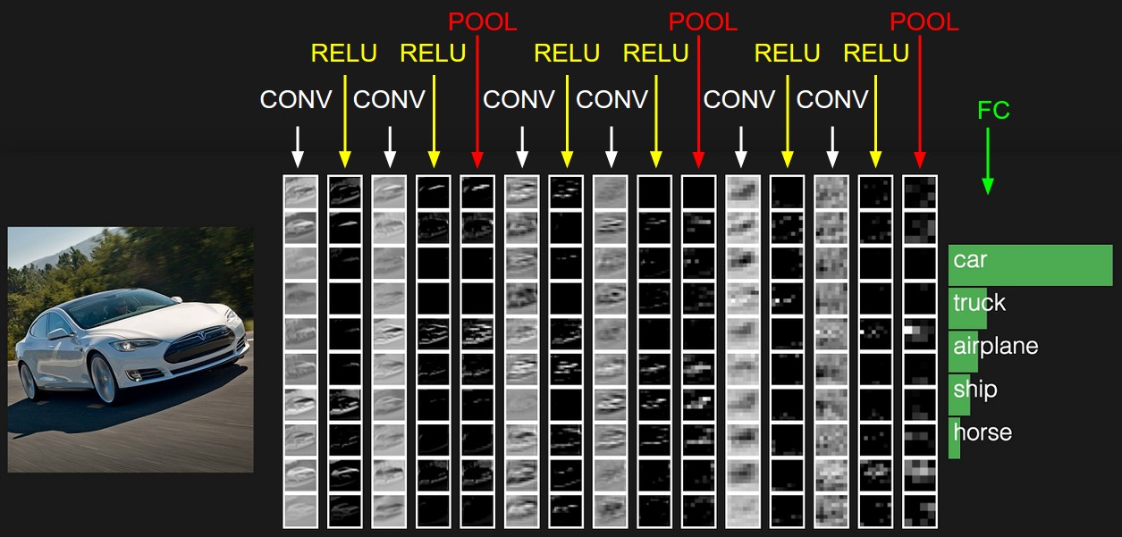
I experimented alot and after some literature research I was inspired by the VGG-design (http://cs231n.github.io/assets/cnn/convnet.jpeg & https://arxiv.org/pdf/1409.1556.pdf)
My final model consisted of the following layers:
| Layer | Description | Comment |
|---|---|---|
| Input | 32x32x3 RGB image | |
| Convolution 1x1 with RELU | 1x1 stride, same padding, outputs 32x32x3 | Here the CNN can train how to use a different combinations of colors |
| Convolution 5x5 with RELU | 1x1 stride, same padding, outputs 32x32x32 | Layer1 |
| Convolution 5x5 with RELU | 1x1 stride, same padding, outputs 32x32x32 | Layer2 |
| Max pooling | 2x2 stride, outputs 16x16x32 | |
| DROPOUT | ||
| Convolution 5x5 with RELU | 1x1 stride, same padding, outputs 16x16x64 | Layer3 |
| Convolution 5x5 with RELU | 1x1 stride, same padding, outputs 16x16x64 | Layer4 |
| Max pooling | 2x2 stride, outputs 8x8x64 | |
| DROPOUT | ||
| Convolution 5x5 with RELU | 1x1 stride, same padding, outputs 8x8x128 | Layer5 |
| Convolution 5x5 with RELU | 1x1 stride, same padding, outputs 8x8x128 | Layer6 |
| Max pooling | 2x2 stride, outputs 4x4x128 | |
| DROPOUT | ||
| Flatten Layer2&4&6 | ||
| Concat Layer2&4&6 | outputs 1x1x14336 | |
| Fully connected with RELU | outputs 1024 | FC1 |
| DROPOUT | ||
| Fully connected with RELU | outputs 512 | FC2 |
| DROPOUT | ||
| Fully connected | outputs 43 | classes output |
As you can see, the information from the lower levels is also transferred to the level of fully connected layers. By doing this, the fully connected layers have access also to low level features, which is very good for simple shapes like traffic signs.
3. Describe how you trained your model. The discussion can include the type of optimizer, the batch size, number of epochs and any hyperparameters such as learning rate.
To train the model, I used an the Adam Optimizer.
Different hyperparameters were tested, these ones seem to be quite good:
- EPOCHS = 100
- BATCH_SIZE = 128
- start_learning_rate = 0.0015
- final_learning_rate = 0.0002
- keep_prob = 0.47
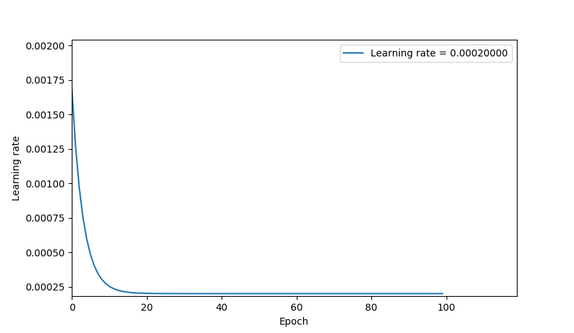
The learning is lowered each epoch according to the formula, which looks something like below:
learning_rate_epoch = start_learning_rate * np.exp(-i*(1/(EPOCHS*0.03))) + final_learning_rate
A L2 LossRegularizer was used to punish big weights. Method: All weights from all layers were summed up and added to the loss operation.
- regularize_factor = 0.00005
The Regularization formula is:
loss_operation = tf.reduce_mean(cross_entropy) + regularize_factor * regularizers
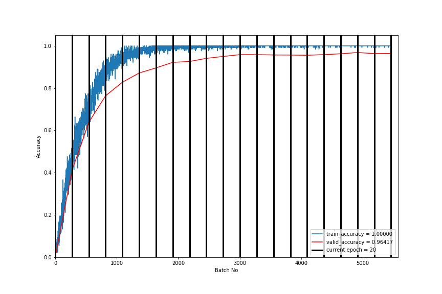
I build a visualization to follow the training progress better, it costs more time, but it is very helpful for detecting under/overfitting, bugs etc. It looks something like this:
My final model results were:
- Validation set accuracy of 98,9 %
- Test set accuracy of 97,9 %
4. Describe the approach taken for finding a solution and getting the validation set accuracy to be at least 0.93. Include in the discussion the results on the training, validation and test sets and where in the code these were calculated. Your approach may have been an iterative process, in which case, outline the steps you took to get to the final solution and why you chose those steps. Perhaps your solution involved an already well known implementation or architecture. In this case, discuss why you think the architecture is suitable for the current problem.
Iterative steps (Hyperparameter tuning in between: lowering learning rate, increasing EPOCHS, etc..):
- Original LeNet with gray images (accuracy not good enough)
- Color LeNet (3 Colorchannels) with colored images (getting around 93% accuracy, not good enough, probably underfiting)
- Color LeNet with colored images and also augmented data set(getting around 94% accuracy, not good enough, probably underfiting)
- Modified Color LeNet (additional Conv Layer and increased depth) with colored images and also augmented data set(getting around 96% accuracy... we can do better)
- Literature research
- CNN inspired by VGG Net (additional Conv Layers, stacking Conv Layers, increased depth and Dropout, L2 Regularization) with colored images and also augmented data set (getting around 98% accuracy)
- took much longer to train, but getting valid accuracy up to 99%
- small learning rate is essential, especially when getting to the ragion of >96%
- dropout is important for avoiding overfitting
- L2 weight regularization is also used to avoid overfitting
After getting validation accuracy > 98%, I checked every epoch if the current validation accuracy is greater than 0.98 and if so, save the current CNN. With this strategy I got the best CNN CNN_final_0.98889 and used this for the next task. This CNN can be found here. Training took about 30-45 without plotting, my workhorses is a Geforce GTX 1060 6GB.
Test a Model on New Images
1. Choose five (I did 12) German traffic signs found on the web and provide them in the report. For each image, discuss what quality or qualities might be difficult to classify.
Here are the 12 German traffic signs that I found on the web:
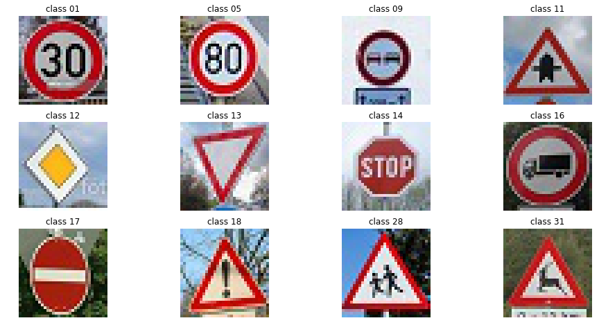
These signs should be classified correctly, I can't see what would cause a problem.
2. Discuss the model's predictions on these new traffic signs and compare the results to predicting on the test set. At a minimum, discuss what the predictions were, the accuracy on these new predictions, and compare the accuracy to the accuracy on the test set
The best CNN CNN_final_0.98889 was restored and used. Here are the results of the prediction:
| Target class | class Prediction |
|---|---|
| 1 | 1 |
| 5 | 5 |
| 9 | 9 |
| 11 | 11 |
| 12 | 12 |
| 13 | 13 |
| 14 | 14 |
| 16 | 16 |
| 17 | 17 |
| 18 | 18 |
| 28 | 28 |
| 31 | 31 |
The model was able to correctly guess 12 of the 12 traffic signs, which gives an accuracy of 100%.
3. Describe how certain the model is when predicting on each of the five new images by looking at the softmax probabilities for each prediction. Provide the top 5 softmax probabilities for each image along with the sign type of each probability. (OPTIONAL: as described in the "Stand Out Suggestions" part of the rubric, visualizations can also be provided such as bar charts)
All images can be classified correctly.
Here are two examples for good classifications, on the first image the CNN is 100% sure and class is correct! This is an excellent result. For the other image the CNN is a bit unsure, but this is just a very small uncertainty.
