
This project builds on the first project, but now uses advanced method of finding lines. The aim of this project is to write a robust lane line finding algorithm to deal with complex senarios like curving lines, shadows and changes in the color of the pavement.
Images from the videos, which are used in this project (SDCND-P4_Advanced-Lane-Lines.ipynb) can be found here(mega.nz link)
Results (Youtube link):
The goals / steps of this project are the following:
- Calibration & Edge Enhancement
- Compute the camera calibration matrix and distortion coefficients given a set of chessboard images
- Apply a distortion correction to raw images
- Apply a edge enhancement to the images
- Warping & cutting image
- Warp with a perspective transform ("birds-eye view")
- Cut out unnecessary parts of the image
- Getting Binary
- Getting the binary thresholded image by using color transforms, gradients, etc.
- Getting Lane Lines: Polyfit using sliding window
- Detect lane pixels and fit to find the lane boundary using the sliding window method
- Getting Lane Lines: Polyfit using previous fit search window
- Detect lane pixels and fit to find the lane boundary using the search window method
- Get meter per pixel
- Determine how much meter per pixel by using the distance from left to right lane line and dashed line length
- Measure Curvature and draw on real image
- Determine the curvature of the lane and vehicle position with respect to center
- Warp the detected lane boundaries back onto the original image
- Complete Pipeline
The OpenCV functions "cv2.findChessboardCorners" and "cv2.calibrateCamera" are used to calculate the correct camera matrix and distortion coefficients using the calibration chessboard images provided in the repository. This data is stored in a .p-file "calibration_file.p" for convenience and speed. The distortion matrix is then used to un-distort the images with the function "cv2.undistort". A slight edge enhancement method is also used, kernel comes from: "OpenCV with Python By Example by Prateek Joshi". Look at the white car in the second image to see this effect.
kernel = np.array([[-1,-1,-1,-1,-1],
                     [-1,2,2,2,-1],
                     [-1,2,8,2,-1],
                     [-1,2,2,2,-1],
                     [-1,-1,-1,-1,-1]]) / 8

output = cv2.filter2D(img,-1,kernel)
Examples of undistorted and edge enhanced images :


The OpenCV function "cv2.getPerspectiveTransform" is been used to correctly rectify each image to a "birds-eye view". As the method of interpolation "cv2.INTER_NEAREST" gives the best result for my pipeline. The source and destination points are hand-tuned to the two images with straight lines. The perspective transformed image of straight lines should have lane lines that are close to being ‘parallel’ to one another. This is because the lane lines are equidistant from one another, so it should maintain this equidistance throughout the warped image. This resulted in the following source and destination points:
| Source | Destination | Comment |
|---|---|---|
| 696, 455 | 930, 0 | top right |
| 587, 455 | 350, 0 | top left |
| 235, 700 | 350, 720 | bottom left |
| 1075, 700 | 930, 720 | bottom right |
example:

Then a "region of interest"-mask is used to cut out unnecessary areas ("cv2.fillPoly"), but keep enough of the image to see sharp curves, example:
 All of the above functions are summarized in a function called "preprocess_img", which undistorts, warps to bird-eye-view and than enhances the edges of the images
This part is the most complex in the pipeline. The most important thing is: Different thresholding methods are used on the image and then a voting between these methods is done. Every method is split into recognizing yellow(yel) and white(wht) lines. This enables the algorithm (if used only on small windows of the image as described later) to detect the color of a line and once this is done, only look for the specified color. Used methods are:
- colormask threshold on HLS, HSV, LAB and red versions of the image; the tresholds are adaptive to the mean of the given image or window of image
- cv2.adaptiveThreshold is fed with multiple 1-channel images and then these masks are connected with the Boolean AND
- for white it is fed with the R-channel of the original image and the V-channel of the HSV image
- for yellow it is fed with the S-channel of the HLS image and the B-channel of the LAB image
So in the end 5 different masks (HLS mask, HSV mask, LAB mask, red mask and adaptive mask) are generated, for the result they are added up numerically and every pixel which has a value smaller 3 is set to 0 and every pixel which has a value bigger or equal 3 is set to 1 to get a normal binary image. The adaptive Threshold vote gets counted twice. These images should illustrate the procedure:
H L S channels and mask:

H S V channels and mask:

L A B channels and mask:

red channel and adaptive threshold mask:

original image with boundaries for adaptive threshold, all masks combined, adaptive threshold mask:

First a histogram along all the columns in the lower half of the image is taken. With this histogram I am adding up the pixel values along each column in the image. In my thresholded binary image, pixels are either 0 or 1, so the two most prominent peaks in this histogram will be good indicators of the x-position of the base of the lane lines. I use that as a starting point for where to search for the lines. From that point, I use a sliding window, placed around the line centers, to find and follow the "hot" pixels up to the top of the frame. These pixels are then used to polyfit a second order polynomial to the following formula:

We're fitting for f(y), rather than f(x), because the lane lines in the warped image are near vertical and may have the same x value for more than one y value.
The following parameters were chosen:
# Choose the number of sliding windows
nwindows = 10
# Set the width of the windows +/- margin
margin = 75
# Set minimum number of pixels found to recenter window
minpix = 45
We can calculate the polynomial data with the formula above for y = 0 : ysize; ysize = 720. With that, for every y-position we have a x-position. In the image below the white line represents this polynomial data, red are hot left line pixels, blue are hot right line pixels:

Now you know where the lines are you have a fit! In the next frame of video it isn't necessary to do a blind search again, but instead just search in a margin around the previous line position like this:

One big problem to overcome are images with bright road and shadows. This urges for a method to adapt the tresholds to small windows of the image. So a method was implemented on top of the getting_binary-function: Once a full image is analyzed and the polyfit is done using the previous method from 4., split the following image into a number of windows, which follow the course of the old polyfit.
Then feed these small windows successively to the getting_binary-function and adapt the thresholds of the binary methods to the mean of each small window. Put all the small binary windows back together to one binary image with full size.
To do this all the polynomial data from one frame to the next must be known, so all data (x- and y-values of the polynomial curve) are stored in a global variable called poly_arr. This variable can also be used to smooth/average the poly-curve from one frame to the next. I chose to smooth with the moving average from the 6 last frames.
poly_data = np.array([left_fitx, right_fitx, ploty])These parameters were chosen:
# Set the width of the windows for the binary image and for the search window; +/- margin
bin_win_margin = 75
margin = 60

# Choose the number of binary windows
nwindows = 10

# Set number of averaging frames
avg_no_frames = 6
Another advantage is that you can only look for the color (white or yellow), which got recognized in the last frame on corresponding line side. This cancels out some noise. Visualization of this method:

For determing the curvature you need to know how many meters one pixel in the "birds-eye" view has. This involves measuring how long and wide the section of lane is that we're projecting in our warped image. To derive a conversion from pixel space to world space, compare the images with U.S. regulations that require a minimum lane width of 12 feet or 3.7 meters, and the dashed lane lines are 3.048 meters long each.
![]()
That gives us:
averaged meter per pixel in y direction : ym_per_pix = 0.02032
averaged meter per pixel in x direction : xm_per_pix = 0.00873164519029
The radius of curvature (awesome tutorial here) at any point x of the function x=f(y) is given as follows:

In the case of the second order polynomial above, the first and second derivatives are:


So, our equation for radius of curvature becomes:

The y values of your image increase from top to bottom, so if, for example, you wanted to measure the radius of curvature closest to your vehicle, you could evaluate the formula above at the y value corresponding to the bottom of your image, or in Python, at yvalue = image.shape[0].
We've calculated the radius of curvature based on pixel values, so the radius we are reporting is in pixel space, which is not the same as real world space. So we actually need to repeat this calculation after converting our x and y values to real world space.
# Fit new polynomials to x,y in world space
left_fit_corrected = np.polyfit(ploty*ym_per_pix, left_fitx*xm_per_pix, 2)
right_fit_corrected = np.polyfit(ploty*ym_per_pix, right_fitx*xm_per_pix, 2)
# Calculate the new radii of curvature
left_curverad = ((1 + (2*left_fit_corrected[0]*y_eval*ym_per_pix + left_fit_corrected[1])**2)**1.5) / np.absolute(2*left_fit_corrected[0])
right_curverad = ((1 + (2*right_fit_corrected[0]*y_eval*ym_per_pix + right_fit_corrected[1])**2)**1.5) / np.absolute(2*right_fit_corrected[0])
# Now we have radius of curvature in meters
example:

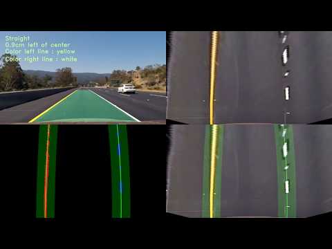
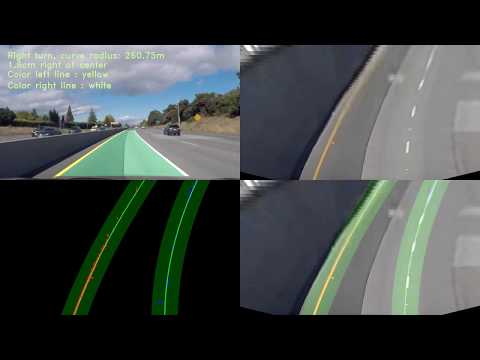
A complete image processing pipeline was established to find the lane lines in images successfully and can process videos frame by frame. The video output project_video_output.mp4 and challenge_video_output.mp4 can be found in this directory.
Example of pipelined frame with debugging views:

The problems I encountered were almost exclusively due to lighting conditions, shadows, discoloration, etc. It wasn't difficult to dial in threshold parameters to get the pipeline to perform well on the original project video (particularly after discovering the B channel of the LAB colorspace, which isolates the yellow lines very well), even on the lighter-gray bridge sections that comprised the most difficult sections of the video.
The challenge video was harder, because of very bad lighting conditions. To also succed in the challenge video I had to come up with the mentioned method of binary windows. This works acceptable on the challenge video, but not perfect. Also it seems that the camera mounting in the challenge video is different, which causes some perspective problems.
Another problem occurs when no dashed line is detected near the front of the car and the line is going sideways. One strategy could be to come up with "anchor-points" that are located at y = ysize - 20 pixel(hood) = 700, so where the line hits the car front. This crossings points should only change slightly if the car is not changing lanes. This approach could also be used to invalidate poly-fits if the left and right anchor points aren't a certain distance apart (within some tolerance) under the assumption that the lane width will remain relatively constant.
You could also have a look in more sophisticated methods for ORGB: Offset Correction in RGB Color Space for Illumination-Robust Image Processing.
I chose not to used any Sobel operators in this project since I wasn't able to find sobel parameters that worked better than the color thresholding I used. I found that the sobel thresholds are very noisy.
The worst what could happen to my pipeline is something like the harder challenge video where sometimes some lines aren't even visible, then my pipeline detects noise as lines falsely and has a hard time redecting the right line.