With 2 different methods: Classing computer vision using HOG-features & SVM and Using Deep Neural Networks (YOLOv2) enabling real time

Goal: Detect vehicles in a video recorded on a highway.
Chosen methods:
- Classic approach with tools from classic computer vision and machine learning (mainly HOG & Support Vector Machines)
- State of the art Deep Convolution Neural Network YOLOv2
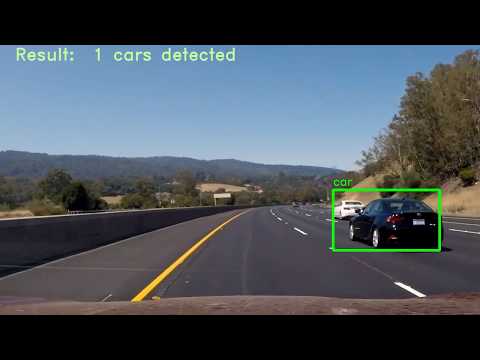
Results (Youtube Links): classic approach:
YOLOv2:
and
In the end both methods were able to detect the vehicles in front of the car, especially the Deep Learning method produec realiably results. The Deep Learning approach enables almost real time detection and tracking with around 15-20 fps on the used machine (1060 6GB GPU). This document describes my approach and implemented pipeline. The code can be found in the corresponding Jupyter Notebooks for the classic approach and YOLOv2.
The steps to achieve these results are the following (you can look up the code from each step under the same chapter number in the notebook:
- Dataset Summary & Exploration
- Feature Extraction 2.1 HOG features 2.2 Spatial binned color features 2.3 Color histogram features 2.4 Complete Feature Extraction pipeline 2.5 Pipeline on dataset 2.6 Normalize features 2.7 Linear dimensionality reduction with PCA
- Training 3.1 Definition of SVM-classifier 3.2 Parameter search 3.3 Final Parameter&Training
- Vehicle detection pipeline 4.1 Multi scale sliding window search for cars 4.2 Heatmap
- Video processing
For the training of the classifier a dataset of images is provided of both cars and "not-cars".
| Class | Count | Shape |
|---|---|---|
| Car | 8792 | 64x64x3 |
| Not-car | 8968 | 64x64x3 |
Info images:
- each image is 12288 pixel (64x64x3)
- every pixel could used as a feature, but training the classifier with that would be higly expensive
- Instead: HOG, color and spatial features
Example image (making sure png and jpg are loaded):

Histogram of Oriented Gradients (HOG): HOG subsamples the image to a grid of e.g. 8x8 or 4x4 pixel grids, with each only containing the most prominent gradient in that part of the image. It therefore extracts gradients in the image while dropping other information like color.
With a color-image you can use all color channels for the HOG-feature. As described later, the LUV-color space was performing best. So below you see the HOG of the 1., 2. and 3. color channel of one car and one not car LUV image:
RGB:

LUV & 3-channel-HOG:


In vector-form this looks something like this:


Spatial binned color features are extracted by downscaling the image and taking the pixel as feature vector. In the downscaling process we reduce the number of pixel significantly but maintain the rough color information of the image. This process is defined in get_hog_features. Example feature vector:
Car
 Not Car

Cars often a dominant color in an image, to capture that numpy.histogram is used to get this feature. Example feature vector
Car
 Not Car

Now we can combine all features to one big feature vector. Its length depends on the parameter we chose for the feature extraction methods above. Example:
Car
 Not Car

This process can be used to vectorize the whole data set as defined in pipeline_dataset.
We have to scale/normalize the feature vector to zero mean and unit variance before training the classifier, because numerically the feature vectors are very different from each other. This was done using sklearn.preprocessing.StandardScaler. After scaling the feature vector looks something like this:

After normalization the dataset is split into train and test set with a ratio 0.8/0.2 using sklearn.model_selection.train_test_split.
After this step the training and test data were saved as a pickle file for later use.
To reduce the number of dimension sklearn.decomposition.PCA was used.
PCA is used to decompose a multivariate dataset in a set of successive orthogonal components that explain a maximum amount of the variance. In scikit-learn, PCA is implemented as a transformer object that learns n components in its fit method, and can be used on new data to project it on these components.
Simply put, it allowed to shrink the feature vector by a factor of 10-20 with only a minor loss in accuracy, see example below. Because the prediction time is highly dependent on the number of features, now the more expensive rbf kernel for the Support Vector Machine kernel can be used.

The extracted features where fed to SVM with a radial basis function kernel (rbf) of sklearn with default setting of square-hinged loss function and l2 normalization.
The trained model along with the parameters used for training were written to a pickle file to be further used by vehicle detection pipeline.
Since this project involves a lot of parameters, I decided to implement an automatic parameter search. These parameters could be tuned:
color_space- used color spaceorient- no of possible HOG orientationspix_per_cell- HOG feature extraction parameterspatial_size- feature extraction parameterhist_bins- feature extraction parameterreduc_factor- Reduction for PCAC- SVM parametergamma- SVM parameterkernel- SVM parameter
These parameters were manually set as the showed the best performance from the beginning:
cell_per_block = 2- HOG feature extraction parameterhog_channel = "ALL"- HOG feature extraction parameter
2 methods were implemented for the automatic parameter search:
-
1. Creating and using a csv-file for a grid-search which can be created by Create_search_space.ipynb. Results with accuracy and speed
-
2. Scikit-Optimize: Bayesian optimization using Gaussian Processes
skopt.gp_minimizewith a customized cost function, to get a good compromise between accuracy and speed:
cost = 25*(1 - accuracy) + time_getting_features/100 + time_prediction_100_samples
Finally these following parameters were chosen, because they performed best:
| Color Space | HOG (orient, pix per cell, cell per block, hog channel) | Color | Histogram | Classifier (kernel, C, gamma) | reduction factor PCA | Accuracy | Prediction time for 100 samples |
|---|---|---|---|---|---|---|---|
| LUV | 19, 16, 2, 'ALL' | (16,16) | 16 | rbf, C=10, 0.005 | n=20 | 0.99718 | 0.051499s |
The detection pipeline scans over an image and uses the trained classifier, normalizer and PCA to detect vehicle in a frame of video.
The pipeline consists of the following steps:
- Calculate HOG feature over entire image and subsample with three different window sizes
- Extract color spatial and histogram features as well
- Normalize and apply PCA to combined feature vector
- Use classifier to predict if there is a car in the subsample
- False positive rejection via heatmap and history
- Annotate found vehicle in input image by drawing a bounding box
The function find_cars from the Udacity lesson material was adopted to allow a multi-scale-search functionality. It applies a trick to the extraction of HOG features. Instead of adjusting the size of the sliding window and then rescaling the subsample back to 64x64 pixel to calculate HOG features, the function is resizing the entire image and calculating HOG features over the entire image. So instead of a 96x96 sliding window that we would have to rescale to 64x64 to calculate HOG features, we scale the entire image down by a factor of 1.5 and subsample with a window size of 64x64.
The image below shows the used region of interest and 3 different scales, which were the input to the function multi_scale_search, which uses the above mentioned function find_cars .
| scale | ystart | ystop |
|---|---|---|
| 1 | 390 | 540 |
| 1.5 | 390 | 615 |
| 2.5 | 390 | 666 |

Next a algorithm/class was implemented to keep a history of a variable amount of frames to only draw bounding boxes when the detection was validated over a few frames. This was done to reject false positives in the video stream. Therefore the concept of heatmap and thresholding was chosen. Also a blur filter was applied to smoothen the results. See class Heatmap for details.
A result of this algorithm is shown below:
 Bottom left: red is history, yellow is validated
For the video each frame was processed according to the above mentioned pipeline.
In this approach darkflow (an tensorflow implementation of darknet & YOLOv2) was used. Setting up the YOLO network was fairly easy, the chosen network configuration was pretrained on the VOC-dataset(which contains a car-class) so a weights file could be loaded. This means that the network didn't need any training at all. These options were chosen:
# define the model options and run
options = {
    'model': 'cfg/yolo-voc.cfg',
    'load': 'bin/yolo-voc.weights',
    'threshold': 0.40,
    'gpu': 0.7,
}
Which gives this network:
Parsing ./cfg/yolo-voc.cfg
Parsing cfg/yolo-voc.cfg
Loading bin/yolo-voc.weights ...
Successfully identified 202704260 bytes
Finished in 0.03650522232055664s
Model has a VOC model name, loading VOC labels.

Building net ...
Source | Train? | Layer description                | Output size
-------+--------+----------------------------------+---------------
       |        | input                            | (?, 416, 416, 3)
 Load  |  Yep!  | conv 3x3p1_1  +bnorm  leaky      | (?, 416, 416, 32)
 Load  |  Yep!  | maxp 2x2p0_2                     | (?, 208, 208, 32)
 Load  |  Yep!  | conv 3x3p1_1  +bnorm  leaky      | (?, 208, 208, 64)
 Load  |  Yep!  | maxp 2x2p0_2                     | (?, 104, 104, 64)
 Load  |  Yep!  | conv 3x3p1_1  +bnorm  leaky      | (?, 104, 104, 128)
 Load  |  Yep!  | conv 1x1p0_1  +bnorm  leaky      | (?, 104, 104, 64)
 Load  |  Yep!  | conv 3x3p1_1  +bnorm  leaky      | (?, 104, 104, 128)
 Load  |  Yep!  | maxp 2x2p0_2                     | (?, 52, 52, 128)
 Load  |  Yep!  | conv 3x3p1_1  +bnorm  leaky      | (?, 52, 52, 256)
 Load  |  Yep!  | conv 1x1p0_1  +bnorm  leaky      | (?, 52, 52, 128)
 Load  |  Yep!  | conv 3x3p1_1  +bnorm  leaky      | (?, 52, 52, 256)
 Load  |  Yep!  | maxp 2x2p0_2                     | (?, 26, 26, 256)
 Load  |  Yep!  | conv 3x3p1_1  +bnorm  leaky      | (?, 26, 26, 512)
 Load  |  Yep!  | conv 1x1p0_1  +bnorm  leaky      | (?, 26, 26, 256)
 Load  |  Yep!  | conv 3x3p1_1  +bnorm  leaky      | (?, 26, 26, 512)
 Load  |  Yep!  | conv 1x1p0_1  +bnorm  leaky      | (?, 26, 26, 256)
 Load  |  Yep!  | conv 3x3p1_1  +bnorm  leaky      | (?, 26, 26, 512)
 Load  |  Yep!  | maxp 2x2p0_2                     | (?, 13, 13, 512)
 Load  |  Yep!  | conv 3x3p1_1  +bnorm  leaky      | (?, 13, 13, 1024)
 Load  |  Yep!  | conv 1x1p0_1  +bnorm  leaky      | (?, 13, 13, 512)
 Load  |  Yep!  | conv 3x3p1_1  +bnorm  leaky      | (?, 13, 13, 1024)
 Load  |  Yep!  | conv 1x1p0_1  +bnorm  leaky      | (?, 13, 13, 512)
 Load  |  Yep!  | conv 3x3p1_1  +bnorm  leaky      | (?, 13, 13, 1024)
 Load  |  Yep!  | conv 3x3p1_1  +bnorm  leaky      | (?, 13, 13, 1024)
 Load  |  Yep!  | conv 3x3p1_1  +bnorm  leaky      | (?, 13, 13, 1024)
 Load  |  Yep!  | concat [16]                      | (?, 26, 26, 512)
 Load  |  Yep!  | conv 1x1p0_1  +bnorm  leaky      | (?, 26, 26, 64)
 Load  |  Yep!  | local flatten 2x2                | (?, 13, 13, 256)
 Load  |  Yep!  | concat [27, 24]                  | (?, 13, 13, 1280)
 Load  |  Yep!  | conv 3x3p1_1  +bnorm  leaky      | (?, 13, 13, 1024)
 Load  |  Yep!  | conv 1x1p0_1    linear           | (?, 13, 13, 125)
-------+--------+----------------------------------+---------------
GPU mode with 0.7 usage
Finished in 32.91464304924011s
The most complicated part was to implement a method to smoothen the detections and delete false positives. Therefore the class car_boxes was implemented in the notebook. This class takes in the box-list as a result from YOLO, compares these box coordinates to all box coordinates in the recorded history (with variable history_depth) and if the current box coordinates are in a relative tolerance (rtol) of one of the history boxes it is validated. These technique allows the track an object. After a variable amount of validated history records(threshold) the box coordinates are considered as a car-box and a moving averaring algorithm is used to smoothen these coordinates.
The algorithm can follow a variable amount of objects (max_no_boxes = 5)
A region of interest (ROI) was also implemented to focus YOLO on the important parts of the video.

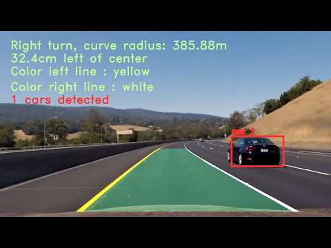
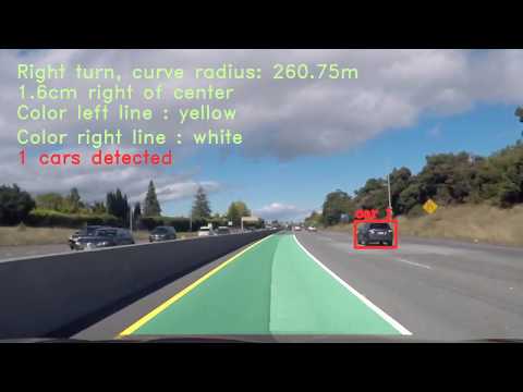
Below you see the pipeline in action with a threshold of 3 (after frame 3, the results are getting validated as car-boxes):
Left is the direct output from yolo | Right is the validated and smoothed result

As one can see the Deep Learning approach was a lot easier to set up, less time-consuming and performed better & faster. Of course it is possible to improve the classic classifier approach by additional data augmentation, negative mining, classifier parameters tuning etc., but it will may fail in case of difficult light conditions and still does not perform in real-time.
The classic approach also has some problems in case of car overlaps another. To resolve this problem one may introduce long term memory of car position and a kind of predictive algorithm which can predict where occluded car can be and where it is worth to look for it.
To even optimize the Deep Learning approach even further, one could train the network on the Udacity Annotated Driving Dataset, but the performance is quite astonishing as it is.
It is a bit unfair to compare the both approaches regarding the real-time capability, because YOLOv2 uses GPU, which has more computational power than the classic approach & CPU. But I would still prefer the Deep Learning approach, because there is no manual fine-tuning of every feature extraction method and training parameter. It just works!
This was a very tedious project which involved the tuning of several parameters by hand. With the traditional Computer Vision approach I was able to develop a strong intuition for what worked and why. I also learnt that the solutions developed through such approaches aren't very optimized and can be sensitive to the chosen parameters. As a result, I developed a strong appreciation for Deep Learning based approaches to Computer Vision. Although, they can appear as a black box at times Deep learning approaches avoid the need for fine-tuning these parameters, and are inherently more robust.