PathPlanningSOS.jl

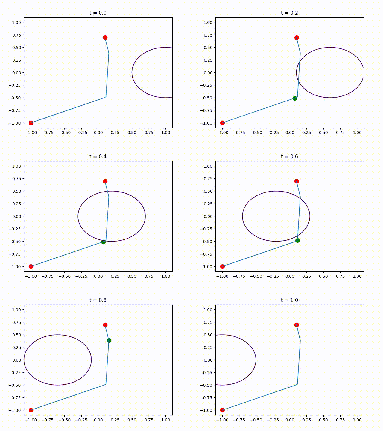
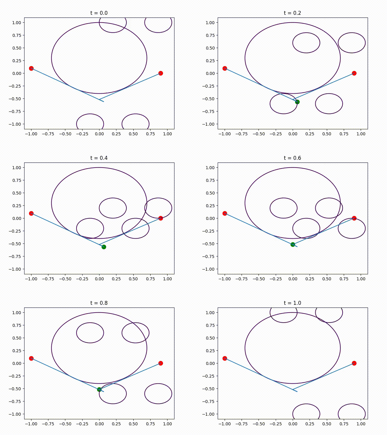
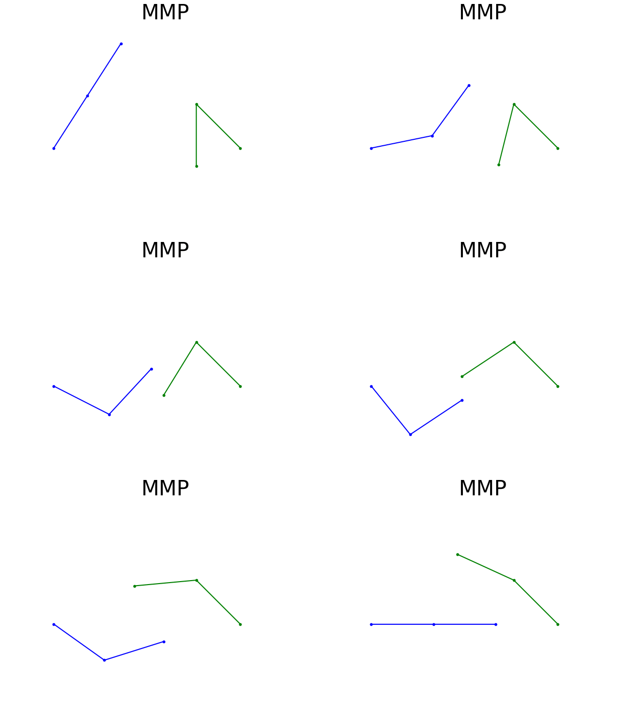
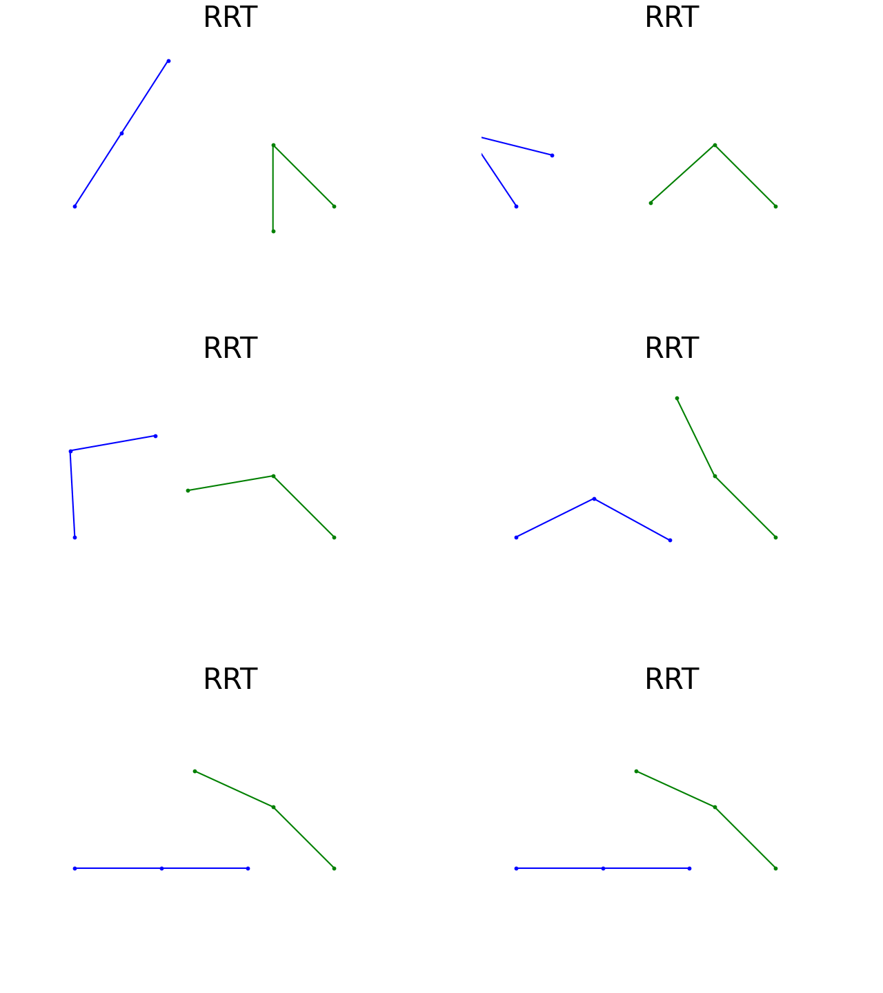
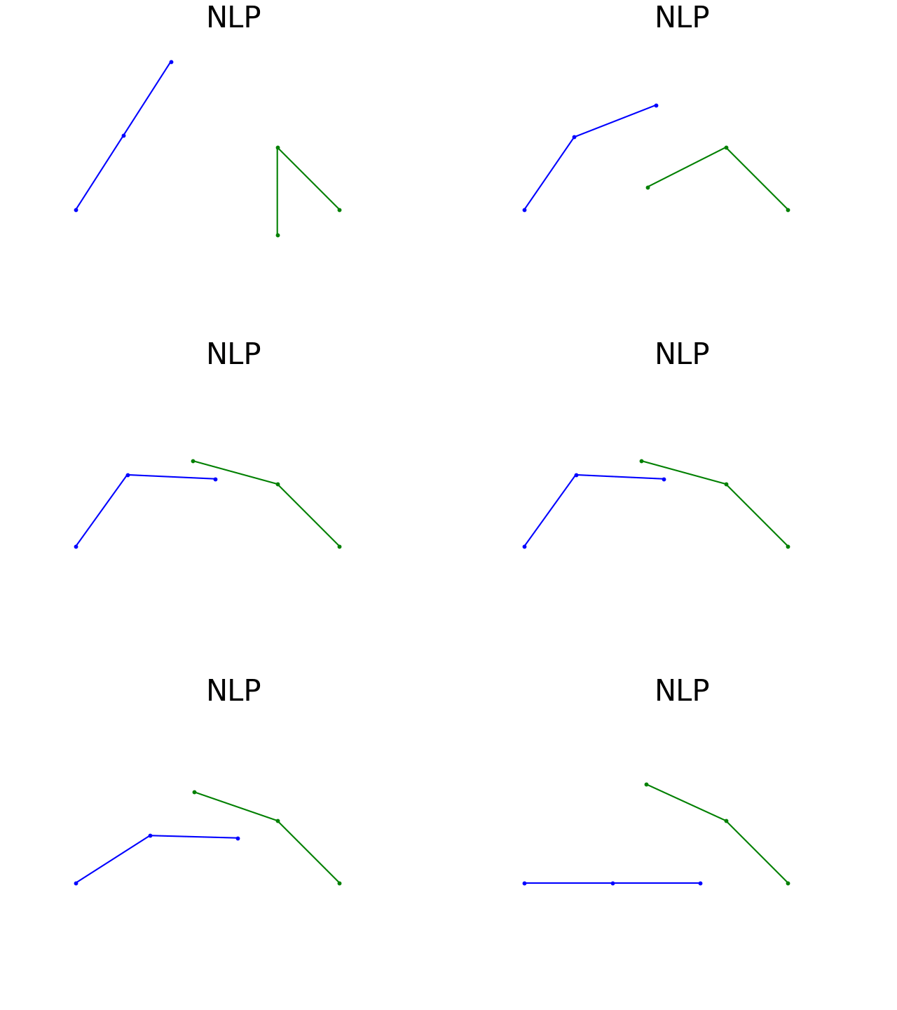
This package contains the code that was used in the numerical experiments of the paper Piecewise-Linear Motion Planningamidst Static, Moving, or Morphing Obstacles.

Abstract: We propose a novel method for planning shortest length piecewise-linear motions through complex environments punctured with static, moving, or even morphing obstacles. Using a moment optimization approach, we formulate a hierarchy of semidefinite programs that yield increasingly refined lower bounds converging monotonically to the optimal path length.

For computational tractability, our global moment optimization approach motivates an iterative motion planner that outperforms competing sampling-based and nonlinear optimization baselines. Our method natively handles continuous time constraints without any need for time discretization, and has the potential to scale better with dimensions compared to popular sampling-based methods.

Proofs. Some numerical experiments.

The role of this package is to find a trajectory (i.e., a continuously-differentiable function) $x: [0, T] \rightarrow \mathbb R^n$ that

starts on a point a and ends on a point b, i.e.
satisfies m obstacle constraints given by inequalities $g_i(t, x(t)) \ge 0$ $\forall t \in [0, T]$ $\forall i \in \{1, \ldots, s\}$

Installation

Open Julia and type-in the following commands to install the required packages.

using Pkg
# download this package
Pkg.add(PackageSpec(url="https://github.com/bachirelkhadir/PathPlanningSOS.jl"))
Pkg.add("JuMP")
Pkg.add("MosekTools") # can be replaced another solver like CSDP or SCS

Example usage

using PathPlanningSOS
using MosekTools
using JuMP

n = 2 # dimension of the space
max_deg_uv = 2 # degree of moment relaxation
num_pieces = 5 # number of linear pieces
num_iterations=20 # number of iterations of the heuristic
weight_lenght= .1 # trade off between minimizing length and rank
random_seed = 3 # random seed used to initialize the heuristic
a = [-1, -1] # starting point
b = [.1, 0.7] # destination
edge_size = 1. # edgesize of the bounding box where the trajectory lives

solver = optimizer_with_attributes(Mosek.Optimizer, "QUIET" => true)

# Obstacle contraints
# here there is a single obstacle: a disk of center [1-2*t, 0] and radius .5
moving_disk = [
    (t, x) -> sum( (x .- [1-2*t, 0]).^2 ) - .5^2
]

# compute optimal piece-wise linear trajectory
opt_trajectory = find_path_using_heuristic(n, moving_disk, edge_size, a, b,
    max_deg_uv, num_pieces, solver,
    weight_lenght,
    num_iterations,
    seed=random_seed)
# opt_trajectory is a function that takes t as input,
# and gives the location of the particle at time t.

Optional

Plot the obtained trajectory.

using PyPlot

# plot setup at time `t`
for (i,t)=enumerate(0:.1:1)
    PyPlot.figure()
    PathPlanningSOS.plot_at_time(t, edge_size, a, b,
                        moving_disk, opt_trajectory)
    PyPlot.title("t = $t")
    fn_index = lpad(i, 3, "0")
    PyPlot.savefig("path_planning_frame_$(fn_index).png")
end

Make a video animation (make sure ffmpeg is installed)

;ffmpeg -r 10 -i path_planning_frame_%03d.png -vcodec libx264 -pix_fmt yuv420p path_planning_animation.mp4 -y

Show video on jupyter notebook

using Base64
base64_video = base64encode(open("path_planning_animation.mp4"))
display("text/html", """<video controls src="data:video/x-m4v;base64,$base64_video">""")

Some Experiments from the Paper