Online, open educational materials for a coastal landscape architecture studio.
Resources Geospatial data sources
Software | GRASS GIS | Rhino |
Tutorials | Intro to GRASS GIS | lecture.lsu.edu/
For our site visit to Elmer's Island on 10/02 please bring a camera, your sketchbook, and as a class a 32"x36" plot with contours and another 32"x36" plot with orthoimagery. Include a north arrow, scale, and cartographic grid on your plots.
Read the
management plan
and its addendum.
As a class compile a list of plants, birds, and terrestrial and marine life
on Elmer's Island.
Then create a library of cutout png images
for at least 10 key species in each category.
Due: 10/06
- Library of plants
- Library of birds
- Library of terrestrial and marine life
As a class build a laser cut contour model of Elmer's Island. Due: 10/13
- Material: museum board (4-ply) or chipboard (1/16" thick)
- Contour interval: 0.25 m
- Tiles: grid of 6 square tiles
As groups of 2 compute geospatial analyses for our site. Work through the terrain analysis and hydrological modeling tutorials. Then design 3 beautiful maps about topics like topography, vegetation, hydrology, sea level rise, and flood risk. Include cartographic elements like legends, labels, scale bars, north arrows, and cartographic grids. Due: 10/13
- 3 maps
- Layout and print all 3 maps on a 36"x72" plot
- Submit digital and print versions
Each group will draw at least 3 sections or section-elevations. Make the section cuts in GRASS GIS or Rhino Based on your site visit, the orthoimagery, and your research illustrate your sections in Photoshop and/or Illustrator to show plant, bird, and marine communities. Due: 10/18
- 3+ illustrated section-elevations
Each group will draw an environmental process diagram and a concept diagram. The first diagram should illustrate how an environmental process like dune morphology, coastal deposition and erosion, land loss, or bird migration functions on Elmer's Island. The concept diagram should highlight what aspect of the site interests you most, explain why it's interesting, and suggest a solution or intervention laying the framework for your first design moves. Due: 10/18
- Environmental process diagram
- Concept diagram
The mid-review will be on 10/23.
There will be a masterplanning charrette on 10/25. In the charrette each team will draw a masterplan and a series of diagrams on trace. Diagrams may include circulation, program, and site systems.
- Hand drawn masterplan
- Hand drawn diagrams
Each group will build a physical conceptual model that develops and explains their driving design idea. For example this model may represent the structure of the boardwalk and it's interface with the land and water, it may show how new planting will shape the future evolution of the dunes, or it may explore how the program will retreat with rising relative sea level.
Each group will build a polymeric sand model their zoomed-in site. Consider using a hollow or inverse contour model to cast the sand model. Then sculpt the sand model with your designed topography.
Each group will develop an illustrative planting plan with a legend describing the plant selection. Each group will also develop a phased scheme for planting over time, which may be represented through sequential plans or axonometrics, sequential sections, or a diagram. Due: 10/20
- Illustrative planting plan
- Phased planting plan or diagram
For the final review on 11/30 curate a selection of your best work representing your site analysis, masterplanning, and site design. You must include a precedent study, a map, a masterplan, a site model, a site plan, an illustrative planting plan, a phased planting plan, 2 sections, and 2 diagrams.
Start GRASS GIS in the nad83_utm15n_barataria location
and create a new mapset called terrain_analysis.
Set your region to our study area with 2 meter resolution using the module g.region by specifying a reference raster map.
g.region raster=elmers_elevation_2m_2012 res=2
Or set your region by specifying its boundaries.
g.region n=3236000 s=3230000 e=788000 w=782000 res=2 save=elmers
Compute contours from the digital elevation model using the module
r.contour
with a 0.1 meter contour interval set with option step=0.1.
Then compute 1 meter contours using the option step=1.
r.contour input=elmers_elevation_2m_2012 output=contours_10cm step=0.1 minlevel=0
r.contour input=elmers_elevation_2m_2012 output=contours_1m step=1 minlevel=0
The contour map will be very noisy.
To reduce the noise,
first smooth the elevation map with
r.neighbors,
then rerun the contour command.
Test different size parameters for r.neighbors.
r.neighbors -c input=elmers_elevation_2m_2012 output=smoothed_elevation size=9
r.contour --overwrite input=smoothed_elevation output=contours_10cm step=0.1 minlevel=0
r.contour --overwrite input=smoothed_elevation output=contours_1m step=1 minlevel=0
Right click on the contour_10cm map layer and select change opacity level.
Set the opacity to 30%.
Right click on the contour_1m map layer and select change opacity level.
Set the opacity to 60%.
Double click on contour_1m in the layer manager,
switch to the line tab,
and make the line weight heavier (eg. 2 or 3 px).
The typical way to visualize hillshading with shaded relief using the module
r.relief
is not very effective for flat landscapes.
Instead use a sky-view factor visualization - a measure of
the openness of the landscape -
using the add-on module
r.skyview.
First call
g.extension
to install the add-on.
The first time you run the add-on with the command r.skyview
you may need to include the flag
--ui to force the graphical user interface to launch.
With the color parameters you can create a colorized sky-view visualization
by draping another map (such as the elevation map) over the sky-view.
Optionally consider using the smoothed elevation as the input.
g.extension extension=r.skyview
r.skyview --overwrite input=elmers_elevation_2m_2012 output=skyview ndir=16 color_source=color_input color_input=elevation_2m_2012 colorized_output=colorized_skyview
Compute the slope and aspect of our study area's topography
using the module
r.slope.aspect.
Optionally change the format from degrees to percent slope
with the parameter format=percent.
Also consider using the smoothed elevation as your input.
r.slope.aspect elevation=elmers_elevation_2m_2012 slope=elmers_slope
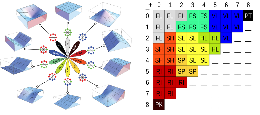
Identify the landforms in our study area using
a machine vision approach based on visibility
with the add-on module
r.geomorphon.
First call
g.extension
to install the add-on.
Then run r.geomorphon --ui to compute basic landforms.
The flag --ui may be needed to force the graphic user interface for the
add-on to launch the first time.
The smoothed elevation will probably generate clearer, more legible results
than the source data elevation.
Experiment with the
search, skip, and flat parameters.
g.extension extension=r.geomorphon
r.geomorphon -m elevation=smoothed_elevation forms=landforms search=50 skip=0 flat=1 dist=0
The landform types are: 1. flat, 2. summit, 3. ridge, 4. shoulder, 5. spur, 6. slope, 7. hollow, 8. footslope, 9. valley, and 10. depression.
Start GRASS GIS in the nad83_utm15n_barataria location
and create a new mapset called viewsheds.
Set your region to our study area with 2 meter resolution using the module g.region by specifying a reference raster map.
g.region raster=elmers_elevation_2m_2012 res=2
Use the module
r.viewshed
to compute a viewshed across the landscape.
The viewshed is what is visible for an observer in a given location.
Optionally change the height of the observer
with the parameter observer_elevation to test views from a new structure like
an observation tower, bird hide, boardwalk, or visitor center.
Again consider using the smoothed elevation as your input.
Experiment with the flags -b or e for different output formats.
r.viewshed input=elmers_elevation_2m_2012 output=viewshed coordinates=785051.917331,3232032.61952 observer_elevation=1.75
Use the add-on module
r.viewshed.cva
to compute the cumulative viewshed for multiple locations.
Create a new vector map called observers.
Use the vector digitizer
 to create observer points.
With the vector digitizer
use the
 digitize new point command to create new points
then quit the digitizer and save your changes.
Use g.extension
to install the add-on.
Then run r.viewshed.cva --ui to run the add-on module.
The flag --ui may be needed to force the graphic user interface for the
add-on to launch the first time.
Use the new vector point map observers as your input vector map.
Optionally change the height of the observers
with the parameter observer_elevation to test views from new structures.
Experiment with the flags -b or e for different output formats.
g.extension extension=r.viewshed.cva
r.viewshed.cva input=elmers_elevation_2m_2012 vector=observers output=cumulative_viewsheds
Start GRASS GIS in the nad83_utm15n_barataria location
and create a new mapset called hydrology.
Set your region to our study area with 2 meter resolution using the module g.region by specifying a reference raster map.
g.region raster=elmers_elevation_2m_2012 res=2
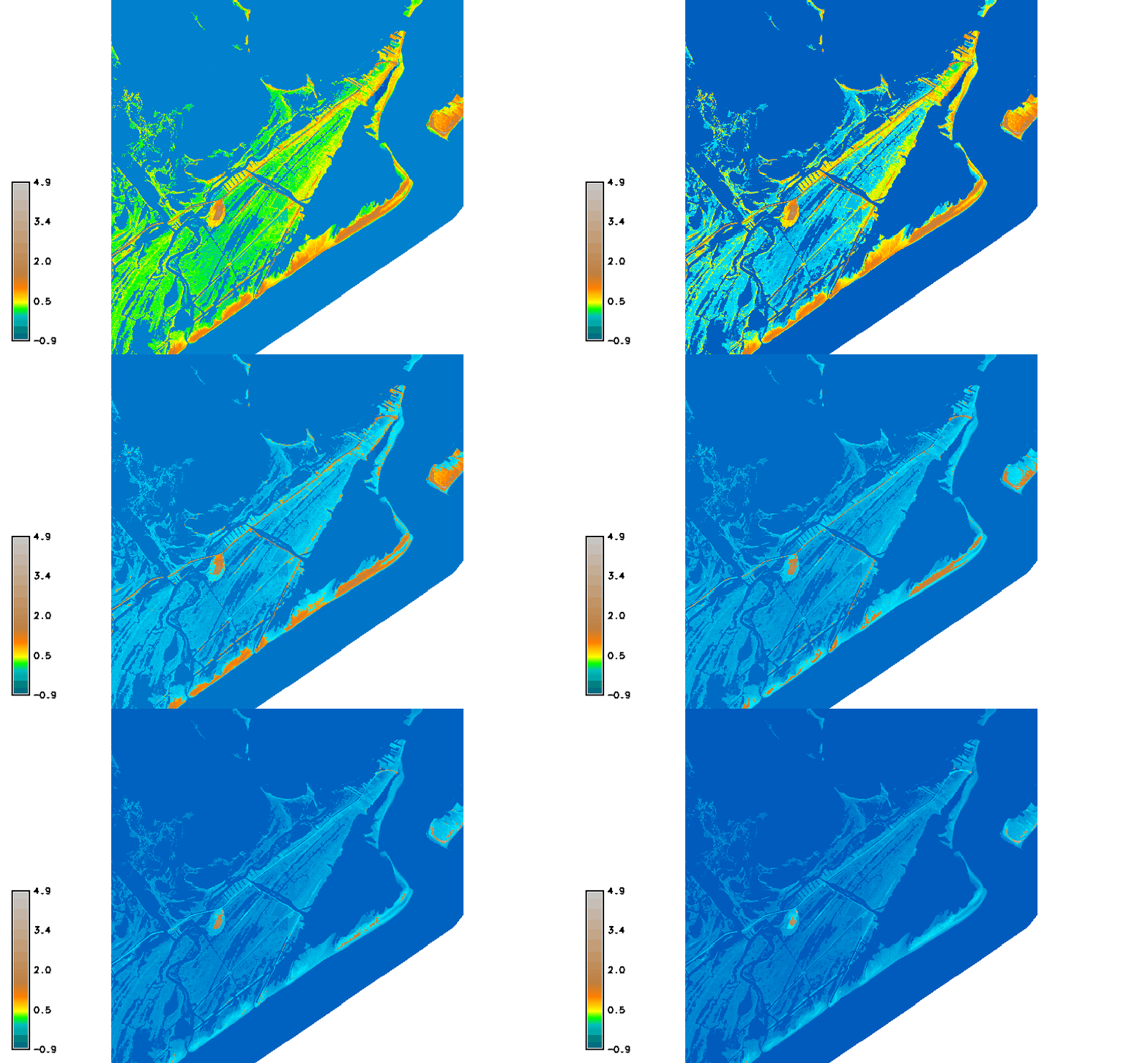
Model current sea level using the module
r.lake.
Set the water level to 0 meter, i.e. sea level.
In the seed tab use the  to pick coordinates somewhere out in the ocean on the map display
for the starting point.
r.lake elevation=elmers_elevation_2m_2012@PERMANENT water_level=0 lake=sea_level
In the layer manager move the sea level map above the elevation and contour maps.
Model flow accumulation for our study area using the module r.watershed.
r.watershed -a elevation=elmers_elevation_2m_2012@PERMANENT accumulation=flow_accumulation
Use map algebra with the GRASS GIS Raster Map Calculator r.mapcalc to remove cells beneath sea level.
r.mapcalc "accumulation = if(isnull(sea_level@PERMANENT),flow_accumulation@hydrology,null())"
This expression means if there are cells where the sea level map is null (ie. has no value), then write the flow accumulation values, else write null values.
Copy the color table from the flow accumulation map using
r.colors
r.colors map=accumulation@hydrology raster=flow_accumulation@hydrology
To see only the concentrated flow accumulation
hide the cells with values less than 60
by either
double clicking on the accumulation map in the layer manager
and setting the list of values to display to 60-58849.4460216767
or running the command:
d.rast map=accumulation@hydrology values=60-58849.4460216767
Experiment to find the right minimum value.
In the layer manager move the accumulation map layer
above the elmers_elevation_2m_2012 and sea_level map layers.
Display the flow accumulation legend
by either pressing the

Add raster legend button
or running the command
d.legend.
Use the -n flag to hide categories
that are not represented in the data.
Install the r.lake.series add-on with
g.extension.
g.extension extension=r.lake.series
Model sea level rise over time using the add-on module
r.lake.series.
In the water tab
set the starting water level to 0 m, the end water level to 2 m,
and the water level step to 0.1 m.
Use the  to pick coordinates somewhere out in the ocean on the map display
for the starting point.
In the time tab set the time step to 5 years
to model sea level rise over 100 years.
This module will create a time series of raster maps
named
 sea_level_rise_0.0, sea_level_rise_0.1, sea_level_rise_0.2, etc...
that will all be registered in a space time raster dataset.
r.lake.series elevation=elmers_elevation_2m_2012@PERMANENT output=sea_level_rise start_water_level=0 end_water_level=2 water_level_step=0.1 coordinates=787832.669323,3232533.86454 time_step=5 time_unit=years
To animate this sea level rise time series launch the GRASS Animation Tool
g.gui.animation.
If you launch the Animation Tool from the File menu in the GUI
follow the these instructions.
Create a new animation,
add a space-time dataset layer,
choose space time raster dataset as the input data type,
and choose the sea_level_rise space time raster dataset.
Then add a raster map layer
and choose elmers_elevation_2m_2012@PERMANENT.
Move this raster map layer beneath the space time raster dataset.
Check the Show raster legend button
and choose elmers_elevation_2m_2012@PERMANENT
as the raster map in the d.legend dialog.
Press Ok to create to the animation.
Press Play to run the animation.
Export your animation as an animated gif.
Press the Export button,
select export to animated GIF,
then browse and name your file,
and press Export.
g.gui.animation strds=sea_level_rise
Upload digital copies of your work to the class network drive
at \\desn-knox.lsu.edu\Landscape-Classes on Windows
or smb://desn-knox.lsu.edu/Landscape-Classes on Mac.
CC BY-SA 4.0 by Brendan Harmon. The license does not apply to logos, fonts, linked material, quotations, or reprinted images by other authors, which may have different licenses. The fonts used in this repository are licensed under the SIL Open Font License by their authors. The syllabus is based on a latex template by Kieran Healy hosted at https://github.com/kjhealy/latex-custom-kjh.


