Max Joseph
August 20, 2016
This document details sparse exact conditional autoregressive (CAR) models in Stan as an extension of previous work on approximate sparse CAR models in Stan. Sparse representations seem to give order of magnitude efficiency gains, scaling better for large spatial data sets.
Conditional autoregressive (CAR) models are popular as prior distributions for spatial random effects with areal spatial data.
If we have a random quantity
where
By Brook's Lemma, the joint distribution of
If we assume the following:
$D_\tau = \tau D$ -
$D = diag(m_i)$ : an$n \times n$ diagonal matrix with$m_i$ = the number of neighbors for location$i$ -
$I$ : an$n \times n$ identity matrix -
$\alpha$ : a parameter that controls spatial dependence ($\alpha = 0$ implies spatial independence, and$\alpha = 1$ collapses to an intrisnic conditional autoregressive (IAR) specification) -
$B = D^{-1} W$ : the scaled adjacency matrix -
$W$ : the adjacency matrix ($w_{ii} = 0, w_{ij} = 1$ if$i$ is a neighbor of$j$ , and$w_{ij}=0$ otherwise)
then the CAR prior specification simplifies to:
The
Suppose we have aggregated count data
where
If we specify a proper CAR prior for
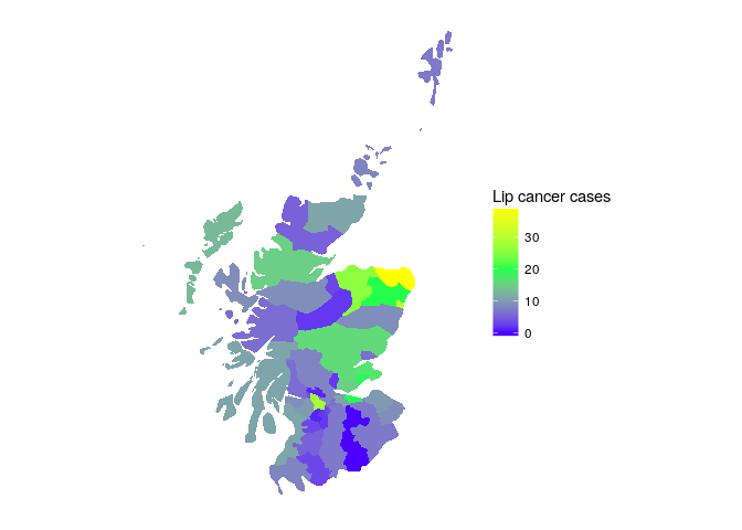
To demonstrate this approach we'll use the Scottish lip cancer data example (some documentation here). This data set includes observed lip cancer case counts at 56 spatial units in Scotland, with an expected number of cases to be used as an offset, and an area-specific continuous covariate that represents the proportion of the population employed in agriculture, fishing, or forestry. The model structure is identical to the Poisson model outlined above.
## Warning in gpclibPermit(): support for gpclib will be withdrawn from
## maptools at the next major release
## [1] TRUE
Let's start by loading packages and data, specifying the number of MCMC iterations and chains.
library(ggmcmc)
library(rstan)
rstan_options(auto_write = TRUE)
options(mc.cores = parallel::detectCores())
source('data/scotland_lip_cancer.RData')

# Define MCMC parameters
niter <- 1E4   # definitely overkill, but good for comparison
nchains <- 4
To fit the full model, we'll pull objects loaded with our Scotland lip cancer data.
I'll use model.matrix to generate a design matrix, centering and scaling the continuous covariate x to reduce correlation between the intercept and slope estimates.
W <- A # adjacency matrix
scaled_x <- c(scale(x))
X <- model.matrix(~scaled_x)

full_d <- list(n = nrow(X),         # number of observations
               p = ncol(X),         # number of coefficients
               X = X,               # design matrix
               y = O,               # observed number of cases
               log_offset = log(E), # log(expected) num. cases
W = W) # adjacency matrixOur model statement mirrors the structure outlined above, with explicit normal and gamma priors on multi_normal_prec function, passing in
data {
  int<lower = 1> n;
  int<lower = 1> p;
  matrix[n, p] X;
  int<lower = 0> y[n];
  vector[n] log_offset;
  matrix<lower = 0, upper = 1>[n, n] W;
}
transformed data{
  vector[n] zeros;
  matrix<lower = 0>[n, n] D;
  {
    vector[n] W_rowsums;
    for (i in 1:n) {
      W_rowsums[i] = sum(W[i, ]);
    }
    D = diag_matrix(W_rowsums);
  }
  zeros = rep_vector(0, n);
}
parameters {
  vector[p] beta;
  vector[n] phi;
  real<lower = 0> tau;
  real<lower = 0, upper = 1> alpha;
}
model {
  phi ~ multi_normal_prec(zeros, tau * (D - alpha * W));
  beta ~ normal(0, 1);
  tau ~ gamma(2, 2);
  y ~ poisson_log(X * beta + phi + log_offset);
}
Fitting the model with rstan:
full_fit <- stan('stan/car_prec.stan', data = full_d,
                 iter = niter, chains = nchains, verbose = FALSE)
print(full_fit, pars = c('beta', 'tau', 'alpha', 'lp__'))
## Inference for Stan model: car_prec.
## 4 chains, each with iter=10000; warmup=5000; thin=1;
## post-warmup draws per chain=5000, total post-warmup draws=20000.
##
## mean se_mean sd 2.5% 25% 50% 75% 97.5% n_eff Rhat
## beta[1] 0.02 0.02 0.29 -0.52 -0.15 0.00 0.16 0.69 321 1.01
## beta[2] 0.27 0.00 0.09 0.08 0.21 0.27 0.34 0.45 3981 1.00
## tau 1.65 0.01 0.50 0.85 1.29 1.59 1.93 2.83 6218 1.00
## alpha 0.93 0.00 0.06 0.77 0.91 0.95 0.98 1.00 3804 1.00
## lp__ 820.81 0.10 6.73 806.63 816.45 821.18 825.52 832.99 4485 1.00
##
## Samples were drawn using NUTS(diag_e) at Thu Feb 9 18:25:48 2017.
## For each parameter, n_eff is a crude measure of effective sample size,
## and Rhat is the potential scale reduction factor on split chains (at
## convergence, Rhat=1).
# visualize results
to_plot <- c('beta', 'tau', 'alpha', 'phi[1]', 'phi[2]', 'phi[3]', 'lp__')
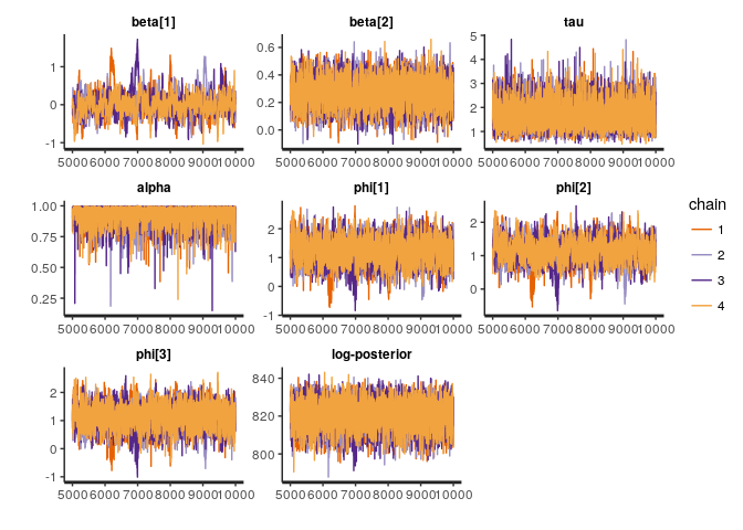
traceplot(full_fit, pars = to_plot)Although we could specify our multivariate normal prior for multi_normal_prec, as we did above, in this case we will accrue computational efficiency gains by manually specifying
In Stan, we only need the log posterior up to an additive constant so we can drop the first term.
Then, substituting
There are two ways that we can accrue computational efficiency gains:
-
Sparse representations of
$\Sigma^{-1}$ to expedite computation of$\phi^T \Sigma^{-1} \phi$ (this work was done by Kyle foreman previously, e.g., https://groups.google.com/d/topic/stan-users/M7T7EIlyhoo/discussion). -
Efficient computation of the determinant. Jin, Carlin, and Banerjee (2005) show that:
where
Again dropping additive constants:
In the Stan model statement's transformed data block, we compute Wsparse), which is assumed to be symmetric, such that the adjacency relationships can be represented in a two column matrix where each row is an adjacency relationship between two sites.
The Stan model statement for the sparse implementation never constructs the precision matrix, and does not call any of the multi_normal* functions.
Instead, we use define a sparse_car_lpdf() function and use it in the model block.
functions {
  /**
  * Return the log probability of a proper conditional autoregressive (CAR) prior
  * with a sparse representation for the adjacency matrix
  *
  * @param phi Vector containing the parameters with a CAR prior
  * @param tau Precision parameter for the CAR prior (real)
  * @param alpha Dependence (usually spatial) parameter for the CAR prior (real)
  * @param W_sparse Sparse representation of adjacency matrix (int array)
  * @param n Length of phi (int)
  * @param W_n Number of adjacent pairs (int)
  * @param D_sparse Number of neighbors for each location (vector)
  * @param lambda Eigenvalues of D^{-1/2}*W*D^{-1/2} (vector)
  *
  * @return Log probability density of CAR prior up to additive constant
  */
  real sparse_car_lpdf(vector phi, real tau, real alpha,
    int[,] W_sparse, vector D_sparse, vector lambda, int n, int W_n) {
      row_vector[n] phit_D; // phi' * D
      row_vector[n] phit_W; // phi' * W
      vector[n] ldet_terms;

      phit_D = (phi .* D_sparse)';
      phit_W = rep_row_vector(0, n);
      for (i in 1:W_n) {
        phit_W[W_sparse[i, 1]] = phit_W[W_sparse[i, 1]] + phi[W_sparse[i, 2]];
        phit_W[W_sparse[i, 2]] = phit_W[W_sparse[i, 2]] + phi[W_sparse[i, 1]];
      }

      for (i in 1:n) ldet_terms[i] = log1m(alpha * lambda[i]);
      return 0.5 * (n * log(tau)
                    + sum(ldet_terms)
                    - tau * (phit_D * phi - alpha * (phit_W * phi)));
  }
}
data {
  int<lower = 1> n;
  int<lower = 1> p;
  matrix[n, p] X;
  int<lower = 0> y[n];
  vector[n] log_offset;
  matrix<lower = 0, upper = 1>[n, n] W; // adjacency matrix
  int W_n;                // number of adjacent region pairs
}
transformed data {
  int W_sparse[W_n, 2];   // adjacency pairs
  vector[n] D_sparse;     // diagonal of D (number of neigbors for each site)
  vector[n] lambda;       // eigenvalues of invsqrtD * W * invsqrtD

  { // generate sparse representation for W
  int counter;
  counter = 1;
  // loop over upper triangular part of W to identify neighbor pairs
    for (i in 1:(n - 1)) {
      for (j in (i + 1):n) {
        if (W[i, j] == 1) {
          W_sparse[counter, 1] = i;
          W_sparse[counter, 2] = j;
          counter = counter + 1;
        }
      }
    }
  }
  for (i in 1:n) D_sparse[i] = sum(W[i]);
  {
    vector[n] invsqrtD;
    for (i in 1:n) {
      invsqrtD[i] = 1 / sqrt(D_sparse[i]);
    }
    lambda = eigenvalues_sym(quad_form(W, diag_matrix(invsqrtD)));
  }
}
parameters {
  vector[p] beta;
  vector[n] phi;
  real<lower = 0> tau;
  real<lower = 0, upper = 1> alpha;
}
model {
  phi ~ sparse_car(tau, alpha, W_sparse, D_sparse, lambda, n, W_n);
  beta ~ normal(0, 1);
  tau ~ gamma(2, 2);
  y ~ poisson_log(X * beta + phi + log_offset);
}
Fitting the model:
sp_d <- list(n = nrow(X),         # number of observations
             p = ncol(X),         # number of coefficients
             X = X,               # design matrix
             y = O,               # observed number of cases
             log_offset = log(E), # log(expected) num. cases
             W_n = sum(W) / 2,    # number of neighbor pairs
             W = W)               # adjacency matrix

sp_fit <- stan('stan/car_sparse.stan', data = sp_d,
               iter = niter, chains = nchains, verbose = FALSE)

print(sp_fit, pars = c('beta', 'tau', 'alpha', 'lp__'))
## Inference for Stan model: car_sparse.
## 4 chains, each with iter=10000; warmup=5000; thin=1;
## post-warmup draws per chain=5000, total post-warmup draws=20000.
##
## mean se_mean sd 2.5% 25% 50% 75% 97.5% n_eff Rhat
## beta[1] -0.01 0.02 0.29 -0.63 -0.15 0.00 0.15 0.57 140 1.03
## beta[2] 0.27 0.00 0.09 0.09 0.21 0.27 0.34 0.46 4449 1.00
## tau 1.64 0.01 0.50 0.86 1.29 1.58 1.94 2.79 5808 1.00
## alpha 0.93 0.00 0.06 0.76 0.91 0.95 0.97 0.99 3169 1.00
## lp__ 782.96 0.10 6.83 768.65 778.50 783.31 787.71 795.26 4418 1.00
##
## Samples were drawn using NUTS(diag_e) at Thu Feb 9 18:26:06 2017.
## For each parameter, n_eff is a crude measure of effective sample size,
## and Rhat is the potential scale reduction factor on split chains (at
## convergence, Rhat=1).
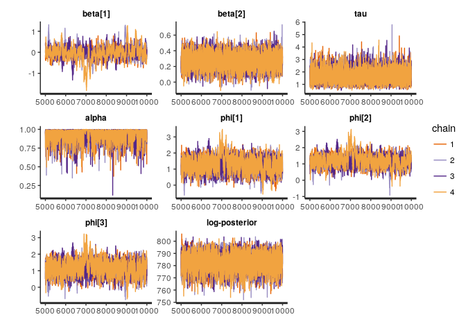
traceplot(sp_fit, pars = to_plot)The main quantity of interest is the effective number of samples per unit time. Sparsity gives us an order of magnitude or so gains, mostly via reductions in run time.
Model Number of effective samples Elapsed time (sec) Effective samples / sec)
full 4485.084 488.56955 9.180032 sparse 4418.415 38.52712 114.683248
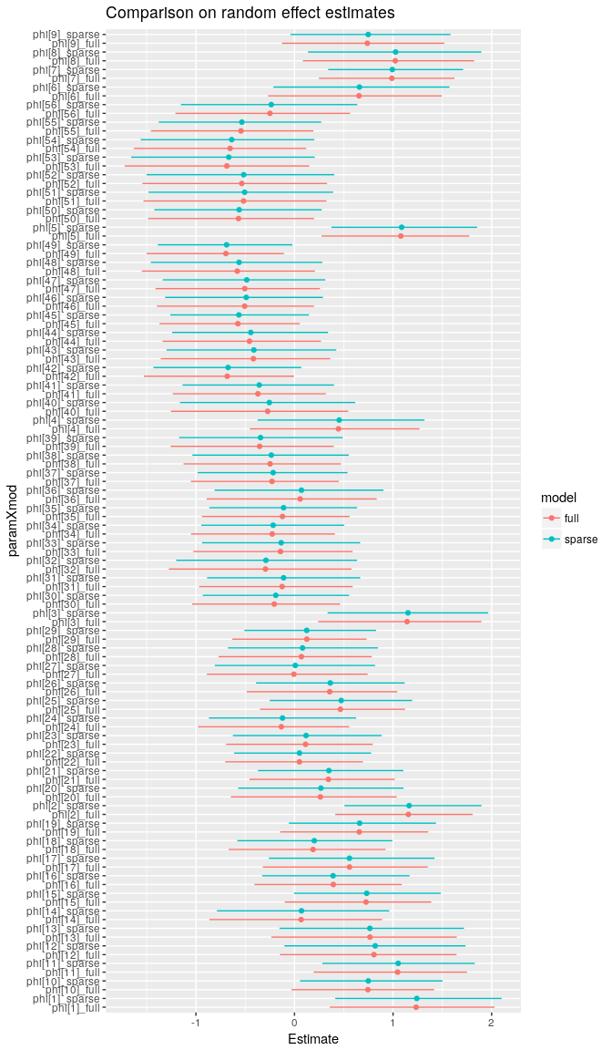
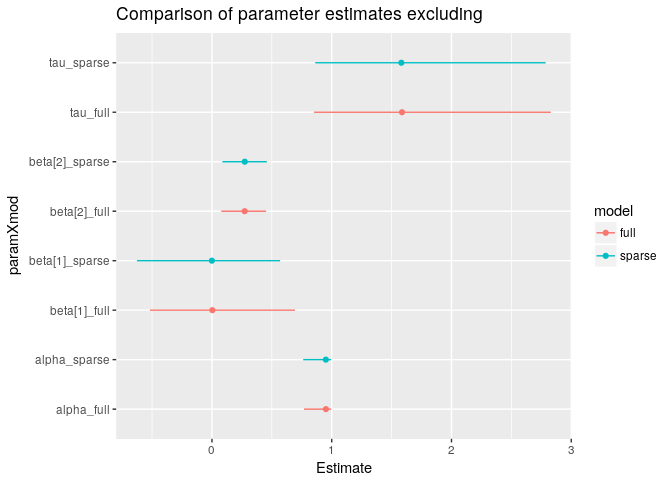
Let's compare the estimates to make sure that we get the same answer with both approaches. In this case, I've used more MCMC iterations than we would typically need in to get a better estimate of the tails of each marginal posterior distribution so that we can compare the 95% credible intervals among the two approaches.
The two approaches give the same answers (more or less, with small differences arising due to MCMC sampling error).
Although the IAR prior for
With
Here
Dropping additive constants, the quantity to increment becomes:
And the corresponding Stan syntax would be:
functions {
  /**
  * Return the log probability of a proper intrinsic autoregressive (IAR) prior
  * with a sparse representation for the adjacency matrix
  *
  * @param phi Vector containing the parameters with a IAR prior
  * @param tau Precision parameter for the IAR prior (real)
  * @param W_sparse Sparse representation of adjacency matrix (int array)
  * @param n Length of phi (int)
  * @param W_n Number of adjacent pairs (int)
  * @param D_sparse Number of neighbors for each location (vector)
  * @param lambda Eigenvalues of D^{-1/2}*W*D^{-1/2} (vector)
  *
  * @return Log probability density of IAR prior up to additive constant
  */
  real sparse_iar_lpdf(vector phi, real tau,
    int[,] W_sparse, vector D_sparse, vector lambda, int n, int W_n) {
      row_vector[n] phit_D; // phi' * D
      row_vector[n] phit_W; // phi' * W
      vector[n] ldet_terms;

      phit_D = (phi .* D_sparse)';
      phit_W = rep_row_vector(0, n);
      for (i in 1:W_n) {
        phit_W[W_sparse[i, 1]] = phit_W[W_sparse[i, 1]] + phi[W_sparse[i, 2]];
        phit_W[W_sparse[i, 2]] = phit_W[W_sparse[i, 2]] + phi[W_sparse[i, 1]];
      }

      return 0.5 * ((n-1) * log(tau)
                    - tau * (phit_D * phi - (phit_W * phi)));
  }
}
data {
  int<lower = 1> n;
  int<lower = 1> p;
  matrix[n, p] X;
  int<lower = 0> y[n];
  vector[n] log_offset;
  matrix<lower = 0, upper = 1>[n, n] W; // adjacency matrix
  int W_n;                // number of adjacent region pairs
}
transformed data {
  int W_sparse[W_n, 2];   // adjacency pairs
  vector[n] D_sparse;     // diagonal of D (number of neigbors for each site)
  vector[n] lambda;       // eigenvalues of invsqrtD * W * invsqrtD

  { // generate sparse representation for W
  int counter;
  counter = 1;
  // loop over upper triangular part of W to identify neighbor pairs
    for (i in 1:(n - 1)) {
      for (j in (i + 1):n) {
        if (W[i, j] == 1) {
          W_sparse[counter, 1] = i;
          W_sparse[counter, 2] = j;
          counter = counter + 1;
        }
      }
    }
  }
  for (i in 1:n) D_sparse[i] = sum(W[i]);
  {
    vector[n] invsqrtD;
    for (i in 1:n) {
      invsqrtD[i] = 1 / sqrt(D_sparse[i]);
    }
    lambda = eigenvalues_sym(quad_form(W, diag_matrix(invsqrtD)));
  }
}
parameters {
  vector[p] beta;
  vector[n] phi_unscaled;
  real<lower = 0> tau;
}
transformed parameters {
  vector[n] phi; // brute force centering
  phi = phi_unscaled - mean(phi_unscaled);
}
model {
  phi_unscaled ~ sparse_iar(tau, W_sparse, D_sparse, lambda, n, W_n);
  beta ~ normal(0, 1);
  tau ~ gamma(2, 2);
  y ~ poisson_log(X * beta + phi + log_offset);
}
Besag, Julian, Jeremy York, and Annie Mollié. "Bayesian image restoration, with two applications in spatial statistics." Annals of the institute of statistical mathematics 43.1 (1991): 1-20.
Gelfand, Alan E., and Penelope Vounatsou. "Proper multivariate conditional autoregressive models for spatial data analysis." Biostatistics 4.1 (2003): 11-15.
Jin, Xiaoping, Bradley P. Carlin, and Sudipto Banerjee. "Generalized hierarchical multivariate CAR models for areal data." Biometrics 61.4 (2005): 950-961.
