temPAWN

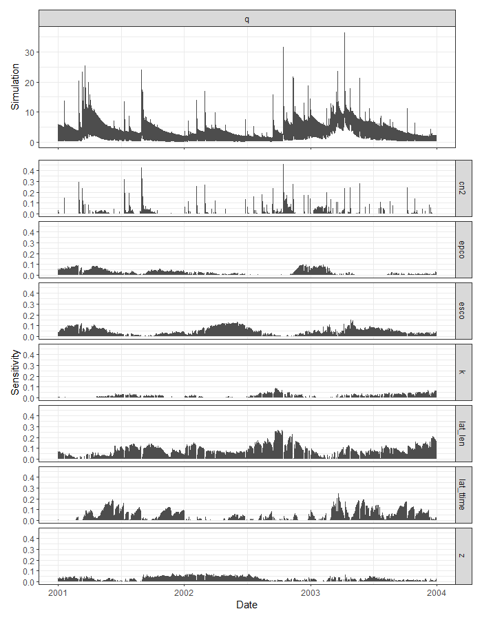
temPAWN calculates the PAWN sensitivity index for each time step of simulation results that were generated with the run_swat*() functions from the SWATplusR package. The PAWN method is implemented according to Pianosi and Wagener (2018). temPAWN optionally includes the computation of the temporal sensitivity of a dummy parameter. Additionally, temPAWN offers a plot function to visualize the sensitivity analysis results.

Installation

You can install the current version of temPAWN from the default branch of the package's GitHub repository:

# If you do not have the package devtools installed
install.packages("devtools")

devtools::install_github("chrisschuerz/temPAWN")

Minimum example

Although "minimum", the example requires quite some computation time. For demonstration, the demo SWAT+ model available from the SWATdata package will be used. In case you do not have SWATplusR and SWATdata installed yet on your computer, you can install both packages via:

devtools::install_github("chrisschuerz/SWATplusR")

devtools::install_github("chrisschuerz/SWATdata")

Run SWAT+ simulations

For the demo we run 1000 SWAT+ simulations to simulate discharge at the demo catchment outlet and y varing 7 model parameters. For further guidance to run SWAT+ simulations in R please see the SWATplusR github page. To generate the 1000 parameter combinations and to run the simulations execute the following lines:

library(SWATplusR)
library(tibble)
library(purrr)
library(lhs)

pth <- load_demo("pro", "set/the/path/where/to/write/the/demo", "plus")

par_bound <- tibble("cn2.hru | change = abschg" = c(-15, 10),
                    "lat_ttime.hru | change = absval" = c(0.5, 50),
                    "lat_len.hru | change = absval" = c(10, 100),
                    "k.sol | change = pctchg" = c(-50, 50),
                    "z.sol | change = pctchg" = c(-50, 50),
                    "esco.hru | change = absval" = c(0, 1),
                    "epco.hru | change = absval" = c(0, 1))

n_sample <- 1000
n_par <- ncol(par_bound)

par_pwn <- randomLHS(n = n_sample, k = n_par) %>%
  as_tibble(., .name_repair = "minimal") %>%
  map2_df(., par_bound, ~ (.x * (.y[2] - .y[1]) + .y[1])) %>%
  set_names(names(par_bound))


sim_pwn  <- run_swatplus(project_path = pth,
                       output = list(q = define_output(file = "channel",
                                                       variable = "flo_out",
                                                       unit = 1)),
                       parameter = par_pwn,
                       start_date = "2000-01-01",
                       end_date = "2003-12-31",
                       years_skip = 1,
                       n_thread = 4)

Analysis with `tempPAWN`

To analyze the performed simulations use the function tempawn(). As the sim argument enter the data object that was returned by run_swatplus(). tempawn() provides additional input arguments for analysis settings. The two most relevant ones are stat and the bins arguments. To understand the effect of these arguments I want to refer to the publication of the PAWN method as it was proposed by Pianosi and Wagener (2018). The analysis is performed as follows:

pwn <- tempawn(sim = sim_pwn)

Visualization of the results

Plotting the temPAWN results works with the function plot(). The result is a visualization of the simulated ranges of the SWAT output variable and the corresponding parameter sensitivities.

plot(pwn)

Plot idea: FDC plots and corresponding parameter sensitivities

An idea that I just had. Generate FDC boundaries of simulated variable and plot the corresponding parameter sensitivities. Line plots are very messy, maybe smooth splines helpful?

References

Pianosi, F. and Wagener T.: Distribution-based sensitivity analysis from a generic input-output sample, Environmental Modelling & Software, 108, 197-207, doi: 10.1016/j.envsoft.2018.07.019, 2018

chrisschuerz/temPAWN