- Python (>=2.7), R
- Python
sklearn,igraphpackages
The C++ files will be build automatically when executing the main script for the first time.
The igraph python package may be installed using the command pip install --user python-igraph
The C++ Windows binaries are already provided, the user does not need to build them.
The igraph python package may be installed by downloading the appropriate pre-compiled binaries found at https://www.lfd.uci.edu/~gohlke/pythonlibs/#python-igraph followed by executing the command python -m pip install desktop/path/igraph.whl
For all platforms, the R dependencies will be installed automatically when executing the main script for the first time.
The goal of this tutorial is to guide the users to use dropClust. Most of the specific parameters have been explained so that users can adjust them specific to particular datasets or as per requirement. An analysis has been described in this tutorial to identify cell type specific genes.
The demo data used for this tutorial has been obtained from https://www.ncbi.nlm.nih.gov/geo/query/acc.cgi?acc=GSE65525 and is provided in a compresssed format (es_mouse.zip).
The provided data must be decompressed to obtain 3 files inside the data/es_mouse folder:
- matrix.mtx, a sparse matrix file containg FPKM values with genes in rows and samples in columns.
- barcodes.tsv, a single column file where each line represents a sampleID corresponding to the matrix columns.
- genes.tsv, a 2 column tab-delimited file where each line contains the (geneID, gene_symbol) correspnding to the matrix rows.
Below is the corresponding Vigenette of the demo_dropClust_main.R file
sourceDir = getwd() # The directory hosting the current script
setwd(sourceDir)
DATA_DIR <- file.path(sourceDir,"data/")
FIG_DIR <-  paste0(sourceDir,"/plots/")
REPORT_DIR  <- paste0(sourceDir,"/report/")
LOUVAIN_DIR <- paste0(sourceDir,"/louvain/")

dir.create(file.path(FIG_DIR),showWarnings = F)
dir.create(file.path(REPORT_DIR),showWarnings = F)
Load relevant libraries & functions for clustering
suppressMessages(source("libraries.R") )
suppressMessages(source("all_functions.R"))
Load data and annotations, the annotations may be omitted if unavailable.
mouse.data<-read10X(file.path(DATA_DIR,"es_mouse/"))
write.csv(x = mouse.data$gene_symbols, file = "gene_symbols.csv",quote = F,row.names =F)
annotation<- read.table(file.path(DATA_DIR,"annotations.csv"),sep = ',',header = T)
ref_id <- as.factor(annotation$x)
dim(mouse.data$mat)
## [1] 2717 24175
Filter poor quality cells. A threshold is provided such that the total UMI count across all genes of the filtered cells is greater than th. th corresponds to the total count of a cell.
filtered.data = filter_cells(mouse.data,th = 5000)## [1] "470 bad cells present."
dim(filtered.data$mat)## [1] 2247 24175
anno_labels= ref_id[filtered.data$keep_cells]
no_samples = dim(filtered.data$mat)[1]
Filter poor genes. Prior to normalization, the function normalize_by_umi_2 filters genes which have UMI count greater than min.count = 2 in atleast min.cell = 3 cells. The dataset containing filtered cells and filtered genes is then UMI normalized.
lnorm<-normalize_by_umi_2(filtered.data, min.count=2, min.cell=3) ## [1] "Dimensions of filtered Matrix:"
## [1] "2247 " "21897 "
For minimising computation load, one third of the total samples is considered with a maximum of 20000 samples. Select Top Dispersed Genes as denoted by ngenes_keep. Write matrix subset to file. The genes are selected based on disperson statsstics.
set.seed(0)

i=min(20000, round(no_samples/3))
sample_ids = sample(1:no_samples, i)

m_n_ngenes <- matrix.subset(lnorm, sample_ids, ngenes_keep = 1000)
## [1] "Select variable Genes..."
## [1] "Sort Top Genes..."
## [1] "Cutoff Genes..."
## [1] "Writing Log Normalized whole_matrix, DIM: 2247 1000 ..."
## [1] "Writing Log Normalized sub_matrix, DIM: 749 1000 ..."
LSH is performend on on 749 samples. This may take some time. Call python script to perform LSH based seach for nearest neighbours and estimate the neighbourhood graph. The default number of neighbours here is set to 10. The neighbourhood graph is partitioned by executing the louvain module in the shell. The present version of dropClust do not support any adjustment of the partition resolution. However the performance of dropClust does not depend on this as long as the scheme can distinguish the smaller group od population in the graph.
call_lsh()## [1] "Reading sparce matrix..."
## [2] ""
## [3] "Converting matrix to dense format..."
## [4] "(749, 1000)"
## [5] "Initialize LSH..."
## [6] "Fit LSH..."
## [7] "Convert into adjacency matrix..."
## [8] "Writing graph edgelist..."
call_louvain()## [1] "Assiging Louvain Communities......................"
Read Louvain clusters for sub-sampling. Specify approximate number of samples to estimate the structure of the data. The samples are expected to sufficiently represent the entire data. The objective is to sample more form the smaller cluster. The optimized_Pinit() function uses simulated anneling to fine tune the exponential decay parameter to obtain the specified set of samples. To ensure selection of sufficient representative transcriptomes from small clusters, the exponential decay function used to determine the proportion of transciptomes to be sampled from each clusteris defined in the sampling() function. The functions had three floating parameters: K, pfin and pinit. The default values are set K=500 and pfin=0.9 and pinit may be optimized to restrict the total number of sub-samples to the user defined value.
opt_pinit = optimized_Pinit(nsamples = 500) ## Initializing par with random data inside bounds
# Sub-sampling using obtained parameter
subsamples_louvain<-sampling(pinit = opt_pinit)
write.csv(x = subsamples_louvain, file = "subsamples_idx",quote = F,row.names =F)
write.csv(x = filtered.data$barcodes[sample_ids[subsamples_louvain]], file = "barcodes_subsamples.csv",quote = F,row.names =F)

# Check the distribution of Sampling across annotated cell types. Skip if annotation is unavailable.
table(anno_labels[sample_ids[subsamples_louvain]])
##
## d0 d2 d4 d7
## 194 59 69 178
The number of samples obtained at this satge subsamples_louvain = 500 may not be an exact match with the input nsamples provided in the optimizer function.
Find PCA top 200 genes. This may take some time.
top_pc_genes<-pc_genes(m_n_ngenes[subsamples_louvain,],top=200) write.csv(x = top_pc_genes, file = "pc_gene_ids_sub.csv",quote = F,row.names =F)Adjust Minimum cluster size with argument minClusterSize (default = 20)
Adjust tree cut with argument level deepSplit (default = 3)
ss_sel_genes_mat<-as.matrix(m_n_ngenes[subsamples_louvain,top_pc_genes])
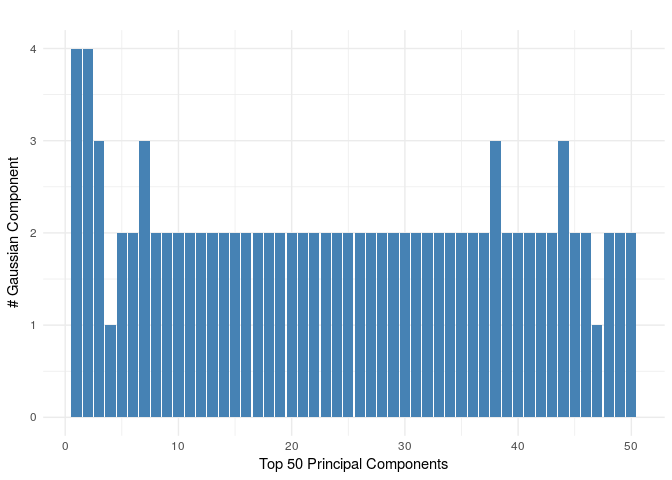
ss_clusters<-ss_clustering(ss_sel_genes_mat, minClusterSize = 20, deepSplit = 3)
## [1] "Predicted Clusters: 5"
The python script calls the LSHforest module to find the approximate K-nearest neighbous of the left put samples. The default value of K here is 5. The neighbours appearing here are among the cells samples previously.
system("python lsh/proj_neigh.py")Class Assignment of Un-annotated cells i.e. the remaining cells which were left out due to sampling. For refwrence, clustering performance on the dropClust samples can be checked at this stage. The final clustering performance is guided by clusters at this stage.
INDEX  = read.csv("neigh.txt",header=F,sep=" ")
dim(INDEX)
## [1] 2247 5
clust_col<-cluster_assign(INDEX, ss_clusters)

write.csv(x = clust_col,file ="predicted.csv", quote = F,row.names = F)

sc_metric(clust_col, as.numeric(anno_labels),show_tab = F) # Skip if annotation is unavailable
## ARI RI Purity
## 0.8572084 0.9366013 0.9327993
Compute Tsne Projection using PCA top genes on the dropClust samples followed by projecting TSNE co-ordinates on the remaining samples.
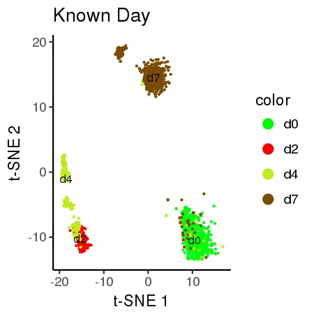
Alert! The known reference labels is for technical demonstration purposes only. The biological significance of the predicted or reference clusters is not known.
PROJ = compute_2d_embedding(data = as.matrix(m_n_ngenes[subsamples_louvain,top_pc_genes]), ss_clusters, INDEX)

dropClust_df<-as.data.frame(cbind(PROJ, clust_col))
rownames(dropClust_df)<-filtered.data$barcodes
save(dropClust_df,file="demo_proj.Rda")


# 2D Vizualization: Known References to Days.
plot_proj_df<-data.frame("Y1" = PROJ[,1],"Y2" = PROJ[,2],color =as.factor(anno_labels))
#plot_proj_df$color <- factor(plot_proj_df$color)
all_plot(plot_proj_df,"known.jpg","Known Day")
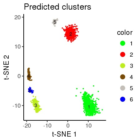
# 2D Vizualization: Predicted Clusters
plot_proj_df_pred<-data.frame(Y1 = PROJ[,1],Y2 = PROJ[,2],color = as.factor(clust_col))
#plot_proj_df_pred$color<-factor(plot_proj_df_pred$color)
all_plot(plot_proj_df_pred,"pred.jpg","Predicted clusters")

