Pure python implementation of Gunnar Farneback's optical flow algorithm
The flow_iterative function is the implementation of the algorithm.
The poly_exp function fits each window of an image to a 2nd order
2D polynomial. Both functions make use of a gaussian applicability
window in order to use separable normalized convolution. This also
allows for certainty to be included as an input to the algorithm.
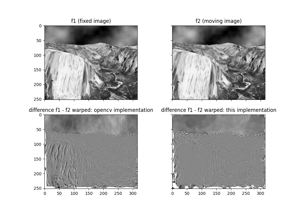
The optical flow method implements an optional affine or projective regularization as described by Farneback. Without the regularization, pixels with low certainty (especially those near edges) tend to have large errors, but the regularization may negatively impact the ability to model local optical flow in the images.
OpenCV implements a similar algorithm described by Farneback. The included script calculates the optical flow on frames from the "Yosemite" sequence using opencv and this algorithm. To install an environment for running this script, use pipenv or conda:
# Run "pipenv lock --dev" or delete Pipfile.lock first if you
# want to solve your own environment
pipenv install --dev
pipenv run pre-commit install  # optionally install pre-commit hooks
pipenv run python compare_to_opencv.py
conda env create
conda activate optical-flow
python compare_to_opencv.pyIn the script, there are two different options for running the algorithm. The first does not regularize the output with a warp parametrization, and the second uses a projective warp regularization. By switching between the options, you can see the differences in the quality of the warp at the edges and at certain interior points with local flow fields.

