NBN4R

NOTE, May 2017 --- some field (column) names in returned data objects may have changed with recent changes to the NBN infrastructure. These are liable to remain in flux but are being investigated.

The National Biodiversity Network (NBN) Atlas provides tools to enable users of biodiversity information to find, access, combine and visualise data on UK and Ireland plants and animals; these have been made available from https://nbnatlas.org/. Here we provide a subset of the tools to be directly used within R.

NBN4R enables the R community to directly access data and resources hosted by the NBN Atlas. Our goal is to enable outputs (e.g. observations of species) to be queried and output in a range of standard formats. This tool is built on the Atlas of Living Australia (ALA4R) package which provides similar services for the ALA. Both NBN and ALA share similar Application Protocol Interface (API) web services. NBN4R wraps ALA4R functions but redirects requests to NBN web servers.

The use-examples based on ALA4R are presented at the 2014 ALA Science Symposium are available in the package vignette, via (in R): vignette("NBN4R"), and a draft modifed version using NBN data is below.

Installing NBN4R

Windows

In R:

Or the development version from GitHub:

install.packages("devtools")
library(devtools)
install_github("fozy81/NBN4R")

You may see a warning about the Rtools package: you don't need to install this. You may also be asked about a location for the R.cache directory --- choose whatever you prefer here, NBN4R does not use R.cache.

If you see an error about a missing package, you will need to install it manually, e.g.:

install.packages(c("stringr","sp"))

and then install_github("fozy81/NBN4R") again.

If you wish to use the data.table package for potentially faster loading of data matrices (optional), also do:

install.packages("data.table")

Linux

First, ensure that libcurl is installed on your system --- e.g. on Ubuntu, open a terminal and do:

sudo apt-get install libcurl4-openssl-dev

or install libcurl4-openssl-dev via the Software Centre.

Then, in R:

Or the development version from GitHub:

install.packages("devtools")
library(devtools)
install_github("fozy81/NBN4R")

If you see an error about a missing package, you will need to install it manually, e.g.:

install.packages(c("stringr","sp"))

and then try installing NBN4R again.

If you wish to use the data.table package for potentially faster loading of data matrices (optional), also do:

install.packages("data.table")

Using NBN4R

The NBN4R package must be loaded for each new R session:

library(NBN4R)

##Customizing NBN4R Various aspects of the NBN4R package can be customized.

###Caching NBN4R can cache most results to local files. This means that if the same code is run multiple times, the second and subsequent iterations will be faster. This will also reduce load on the NBN servers. By default, this caching is session-based, meaning that the local files are stored in a temporary directory that is automatically deleted when the R session is ended. This behaviour can be altered so that caching is permanent, by setting the caching directory to a non-temporary location. For example, under Windows, use something like:

nbn_config(cache_directory <- file.path("c:","mydata","nbn_cache")) ## Windows

or for Linux:

nbn_config(cache_directory = "~/mydata/nbn_cache") ## Linux

Note that this directory must exist (you need to create it yourself).

All results will be stored in that cache directory and will be used from one session to the next. They won’t be re-downloaded from the server unless the user specifically deletes those files or changes the caching setting to “refresh”.

If you change the cache_directory to a permanent location, you may wish to add something like this to your .Rprofile file, so that it happens automatically each time the NBN4R package is loaded:

setHook(packageEvent("NBN4R", "attach"), 
function(...) nbn_config(cache_directory=file.path("~","mydata","nbn_cache")))

Caching can also be turned off entirely by:

nbn_config(caching="off")

or set to “refresh”, meaning that the cached results will re-downloaded from the NBN servers and the cache updated. (This will happen for as long as caching is set to “refresh” — so you may wish to switch back to normal “on” caching behaviour once you have updated your cache with the data you are working on).

###User-agent string Each request to the NBN servers is accompanied by a “user-agent” string that identifies the software making the request. This is a standard behaviour used by web browsers as well. The user-agent identifies the user requests to the NBN, helping the NBN to adapt and enhance the services that it provides. By default, the NBN4R user-agent string is set to “NBN4R” plus the NBN4R version number (e.g. “NBN4R 1.0”).

NO personal identification information is sent. You can see all configuration settings, including the the user-agent string that is being used, with the command:

nbn_config()

###Debugging If things aren’t working as expected, more detail (particularly about web requests and caching behaviour) can be obtained by setting the verbose configuration option:

nbn_config(verbose=TRUE)

Setting the download reason

NBN requires that you provide a reason when downloading occurrence data (via the NBN4R occurrences() function). You can provide this as a parameter directly to each call of occurrences(), or you can set it once per session using:

nbn_config(download_reason_id=your_reason_id)

(See nbn_reasons() for valid download reasons)

Other options

If you make a request that returns an empty result set (e.g. an un-matched name), by default you will simply get an empty data structure returned to you without any special notification. If you would like to be warned about empty result sets, you can use:

nbn_config(warn_on_empty=TRUE)

##Examples First, check that we have some additional packages that we'll use in the examples, and install them if necessary.

to_install <- c("plyr","jpeg","phytools","ape","leaflet","vegan","mgcv","geosphere","maps","mapdata","maptools")
to_install <- to_install[!sapply(to_install,requireNamespace,quietly=TRUE)]
if(length(to_install)>0) install.packages(to_install)

We’ll use the plyr package throughout these examples, so load that now:

library(plyr)

###Example 1: Name searching and taxonomic trees

library(ape)
library(phytools)

We want to look at the taxonomic finches, but we don’t know what the correct scientific name is, so let’s search for it:

sx <- search_fulltext("Finch")
(sx$data[,c("name","rank","family")])

                      name    rank       family
1              Diuca diuca species  Emberizidae
2         Sicalis flaveola species  Emberizidae
3     Rhodopechys obsoleta species Fringillidae
4     Carduelis citrinella species Fringillidae
5     Carpodacus mexicanus species Fringillidae
6  Paludipasser locustella species  Estrildidae
7         Poephila guttata species  Estrildidae
8    Bucanetes githagineus species Fringillidae
9         Amadina fasciata species  Estrildidae
10  Montifringilla nivalis species   Passeridae

And we can see that violets correspond to a number of families. We want to use Estrildidae. Now we can download the taxonomic data (note that the search is case-sensitive):

tx <- taxinfo_download("rk_family:Estrildidae",fields=c("guid","rk_genus","scientificName","rank"))
tx <- tx[tx$rank %in% c("species","subspecies"),] ## restrict to species and subspecies

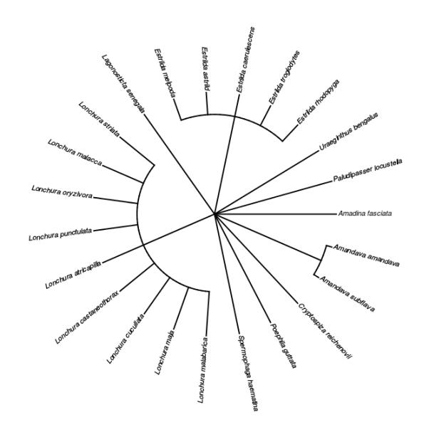
We can make a taxonomic tree plot using the phytools package:

## as.phylo requires the taxonomic columns to be factors
temp <- colwise(factor, c("genus","scientificName"))(tx)
## create phylo object of Scientific.Name nested within Genus
ax <- as.phylo(~genus/scientificName,data=temp)
plotTree(ax,type="fan",fsize=0.7,ftype="i") ## plot it

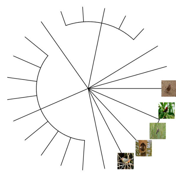
We can also plot the tree with images of the different finches species. We’ll first extract a species profile for each species identifier (guid) in our results:

s <- search_guids(tx$guid)

And for each of those species profiles, download the thumbnail image and store it in our data cache. Unfortunately, not all species have images available. You can browse available images on the NBN Atlas images.

imfiles <- sapply(s$thumbnailUrl,function(z){ 
  ifelse(!is.na(z),NBN4R:::cached_get(z,type="binary_filename"),"") 
})

And finally, plot the tree:

plotTree(ax,type="fan",ftype="off") ## plot tree without labels
tr <- get("last_plot.phylo",envir = .PlotPhyloEnv) ## get the tree plot object
## add each image
library(jpeg)
for (k in which(nchar(imfiles)>0))
        rasterImage(readJPEG(imfiles[k]),tr$xx[k]-1/10,tr$yy[k]-1/10,tr$xx[k]+1/10,tr$yy[k]+1/10)

###Example 2: Quality assertions Data quality assertions are a suite of fields that are the result of a set of tests peformed on NBN data. Download occurrence data for the Blunt-fruited Water-starwort:

x <- occurrences(taxon="Callitriche obtusangula", download_reason_id=10)
summary(x)

# number of original names: 2 
# number of taxonomically corrected names: 1 
# number of observation records: 1319 
# number of assertions listed: 9  -- ones with flagged issues are listed below
# 	invalidCollectionDate: 1 records 
# 	incompleteCollectionDate: 1 records 
# 	precisionRangeMismatch: 1040 records 
# 	firstOfYear: 338 records 
# 	unknownCountry: 474 records 
# 	countryInferredByCoordinates: 806 records 
# 	decimalLatLongCalculatedFromGridReference: 1298 records 
# 	assumedPresentOccurrenceStatus: 992 records 
# 	firstOfMonth: 479 records

There are many other ways of producing spatial plots in R. The leaflet package provides a simple method of producing browser-based maps iwth panning, zooming, and background layers:

library(leaflet)
## drop any records with missing lat/lon values
x$data <- x$data[!is.na(x$data$longitude) & !is.na(x$data$latitude),] 
xa <- check_assertions(x)
## columns of x corresponding to a fatal assertion
x_afcols <- which(names(x$data) %in% xa$occurColnames[xa$taxonIdentificationIssue])
## rows of x that have a fatal assertion
x_afrows <- apply(x$data[,x_afcols],1,any)
## which taxonIdentificationIssue assertions are present in this data?
these_assertions <- names(x$data)[x_afcols]
## make a link to the web page for each occurrence
popup_link <- paste0("<a href=\"https://records.nbnatlas.org/occurrences/",x$data$id,"\">Link to occurrence record</a>")
## colour palette
pal <- c(sub("FF$","",heat.colors(length(these_assertions))))
## map each data row to colour, depending on its assertions
marker_colour <- rep("#00FF00",nrow(x$data))
for (k in 1:length(these_assertions)) marker_colour[x$data[,x_afcols[k]]] <- pal[k]
## blank map, with imagery background
m <- addProviderTiles(leaflet(),"Esri.WorldImagery")
## add markers
m <- addCircleMarkers(m,x$data$longitude,x$data$latitude,col=marker_colour,popup=popup_link)
print(m)

###Example 3: Community composition and turnover Some extra packages needed here:

library(vegan)
library(mgcv)
library(geosphere)

Define our area of interest as a transect running westwards, and download the occurrences of bats:

wkt <- "POLYGON((-3 56,-4 56,-4 57,-3 57,-3 56))"
x <- occurrences(taxon="Vespertilionidae",wkt=wkt,qa="none",download_reason_id=10)
x <- x$data ## just take the data component

Bin the locations into 0.5-degree grid cells:

x$longitude <- round(x$longitude*100)/100
x$latitude <- round(x$latitude*100)/100

Create a sites-by-species data frame. This could also be done with e.g. the reshape library or the table() function, or indeed directly from NBN4R’s species_by_site function. Note: this process inherently makes some strong assumptions about absences in the data.

## discard genus- and higher-level records
xsub <- x$rank %in% c("species","subspecies","variety","form","cultivar")
unames <- unique(x[xsub,]$scientificName) ## unique names 
ull <- unique(x[xsub,c("longitude","latitude")])
xgridded <- matrix(NA,nrow=nrow(ull),ncol=length(unames))
for (uli in 1:nrow(ull)) {
    lidx <- xsub & x$longitude==ull[uli,]$longitude & x$latitude==ull[uli,]$latitude
    xgridded[uli,] <- as.numeric(unames %in% x[lidx,]$scientificName)
}
xgridded <- as.data.frame(xgridded)
names(xgridded) <- unames
xgridded <- cbind(ull,xgridded)

Now we can start to examine the patterns in the data. Let’s plot richness as a function of longitude:

plot(xgridded$longitude,apply(xgridded[,-c(1:2)],1,sum),ylab="Richness",
  xlab="Longitude",pch=20,col="grey25")

The number of species is highest at the eastern end of the transect. This probably reflects both higher species richness as well as greater sampling effort in this area compared to the western end of the transect.

How does the community composition change along the transect? Calculate the dissimilarity between nearby grid cells as a function of along-transect position:

D <- vegdist(xgridded[,-c(1:2)],'bray') ## Bray-Curtis dissimilarity
Dm <- as.matrix(D) ## convert to a matrix object
## calculate geographic distance from longitude and latitude
Dll <- apply(xgridded[,1:2],1,function(z){distVincentySphere(z,xgridded[,1:2])})
closeidx <- Dll>0 & Dll<100e3 ## find grid cells within 100km of each other
## create a matrix of longitudes that matches the size of the pairwise-D matrices
temp <- matrix(xgridded$longitude,nrow=nrow(xgridded),ncol=nrow(xgridded))
## plot dissimilarity as a function of transect position
plot(temp[closeidx],Dm[closeidx],xlab="Longitude",ylab="Dissimilarity",pch=20,
  col="grey85")
## add smooth fit via gam()
fit <- gam(d~s(tp,k=7),data=data.frame(tp=temp[closeidx],d=Dm[closeidx]))
tpp <- seq(from=min(xgridded$longitude),to=max(xgridded$longitude),length.out=100)
fitp <- predict(fit,newdata=data.frame(tp=tpp))
lines(tpp,fitp,col=1)

Clustering:

cl <- hclust(D,method="ave") ## UPGMA clustering
plot(cl) ## plot dendrogram

grp <- cutree(cl,20) ## extract group labels at the 20-group level
## coalesce small (outlier) groups into a single catch-all group
sing <- which(table(grp)<5)
grp[grp %in% sing] <- 21 ## put these in a new combined group
grp <- sapply(grp,function(z)which(unique(grp)==z)) ## renumber groups
## plot
with(xgridded,plot(longitude,latitude,pch=21,col=grp,bg=grp))

## or slightly nicer map plot
library(maps)
library(mapdata)
map("worldHires","UK", xlim=c(-11,3), ylim=c(49,60.9), col="gray90", fill=F)
thiscol <- c("#1f77b4","#ff7f0e","#2ca02c","#d62728","#9467bd","#8c564b",
  "#e377c2","#7f7f7f","#bcbd22","#17becf") ## colours for clusters
with(xgridded,points(longitude,latitude,pch=21,col=thiscol[grp],bg=thiscol[grp],cex=0.75))