Data-Free Knowledge Distillation For Deep Neural Networks

Abstract

Recent advances in model compression have provided procedures for compressing large neural networks to a fraction of their original size while retaining most if not all of their accuracy. However, all of these approaches rely on access to the original training set, which might not always be possible if the network to be compressed was trained on a very large non-public dataset. In this work, we present a method for data-free knowledge distillation, which is able to compress deep models to a fraction of their size leveraging only some extra metadata to be provided with a pretrained model release. We also explore different kinds of metadata that can be used with our method, and discuss tradeoffs involved in using each of them.

Paper

The paper is currently under review for AISTATS 2018 and NIPS 2017 LLD Workshop. You can feel free to read the arxiv or the poster for this work, or contact me with any questions.

Raphael Gontijo Lopes	Stefano Fenu

Overview

Our method for knowledge distillation has a few different steps: training, computing layer statistics on the dataset used for training, reconstructing (or optimizing) a new dataset based solely on the trained model and the activation statistics, and finally distilling the pre-trained "teacher" model into the smaller "student" network. Each of these steps constitute a "procedure", which are implemented in the procedures/ module. Each procedure implements a run function, which does everything from loading models to training.

When optimizing a dataset reconstruction, there's also the choice of different optimization objectives (top layer, all layers, spectral all layers, spectral layer pairs, all discussed in the paper). These are implemented in procedures/_optimization_objectives.py, and take care of creating the optimization and loss operations, as well as of sampling from the saved activation statistics and creating a feed_dict that loads all necessary placeholders.

Every dataset goes under datasets/, and needs to implement the same interface as datasets/mnist.py. Namely, the dataset class needs to have an io_size property that specifies the input size and the label output size. It also needs two iterator methods: train_epoch_in_batches and test_epoch_in_batches.

Note: Credit for the attribute and data files of CelebA dataset is given to this repo.

We provide four models in models/: two fully connected and two convolutional. The fully connected models are hinton-1200 and hinton-800, as described in the original knowledge distillation paper. The convolutional models are LeNet-5, and a modified version of it which has half the number of convolutional filters per layer. Each model implemented to be a teacher network needs to implement all three functions in the interface: create_model, load_model, and load_and_freeze_model. If a model is meant to be a student network, like lenet_half and hinton800, then it need only implement create_model.

Every artifact created will be saved under summaries/, the default --summary_folder. This includes tf summaries, checkpoints, optimized datasets, log files with information about the experiment run, activation statistics, etc.

On the newly added VGG11, 16 and 19 models, there is an option to initialize the layers with ImageNet pre-trained layers. You can get those *.npy files here.

Requirements

This code requires that you have tensorflow 1.0 installed, along with numpy and scikit-image 0.13.0 on python 3.6+.

The visualization scripts (used to debug optimized/reconstructed datasets) also require opencv 3.2.0 and matplotlib.

Usage

Train and Save a Model

First, we need to have the model trained on the original dataset. This step can be skipped if you already have a pre-trained model that you can easily load through the same interface as the ones in models/.

The procedure flag specifies what to do with the model and dataset. In this case, train it from scratch.

python main.py --run_name=experiment --model=hinton1200 --dataset=mnist \
    --procedure=train

Compute and Save Statistics for that Model

We use the original dataset to compute layer statistics for the model. These are the "metadata" mentioned in the paper, which we save so we can reconstruct a dataset representative of the original one.

The model_meta and model_checkpoint flags are required because the compute_stats procedure loads a pre-trained model. If you are planning on optimizing a dataset with a spectral optimization objective, you need to compute stats with the flag compute_graphwise_stats=True. The reason why this is not done by default is because graphwise statistics are computationally expensive.

python main.py --run_name=experiment --model=hinton1200 --dataset=mnist \
    --procedure=compute_stats \
    --model_meta=summaries/experiment/train/checkpoint/hinton1200-8000.meta \
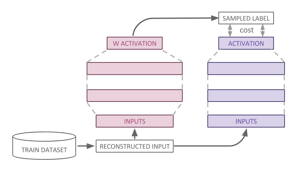
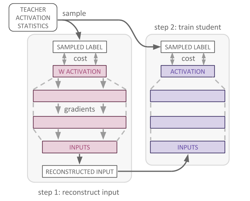
    --model_checkpoint=summaries/experiment/train/checkpoint/hinton1200-8000

Optimize a Dataset Using the Saved Model and the Statistics

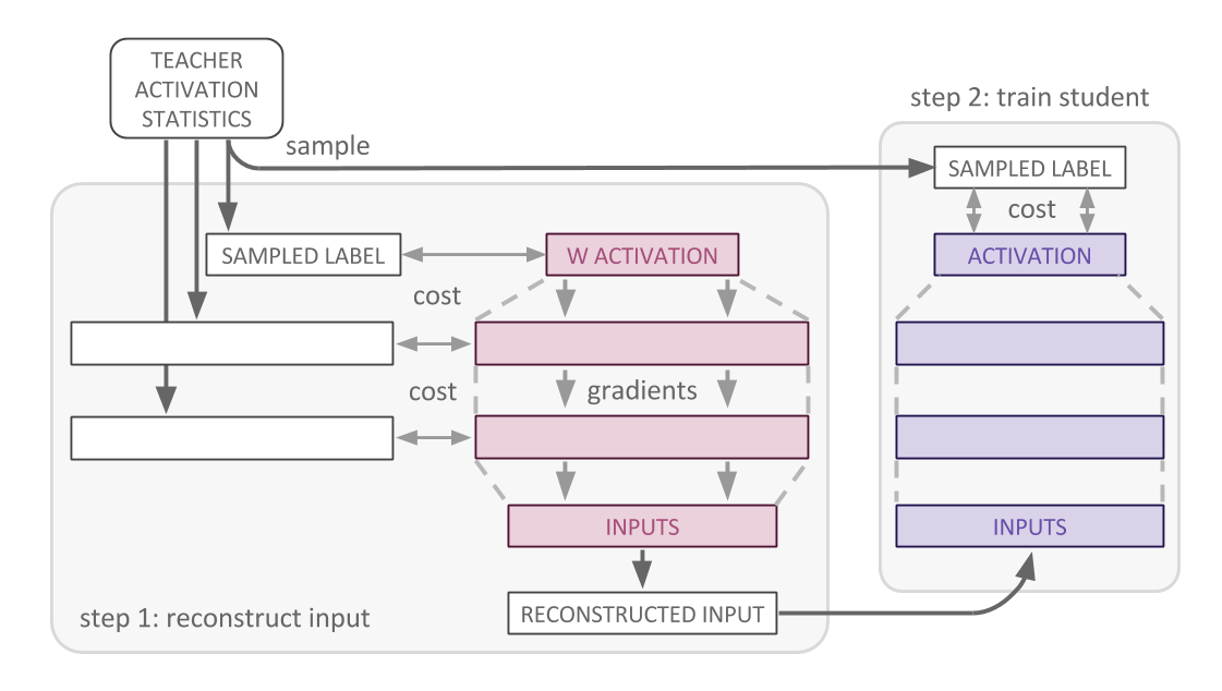
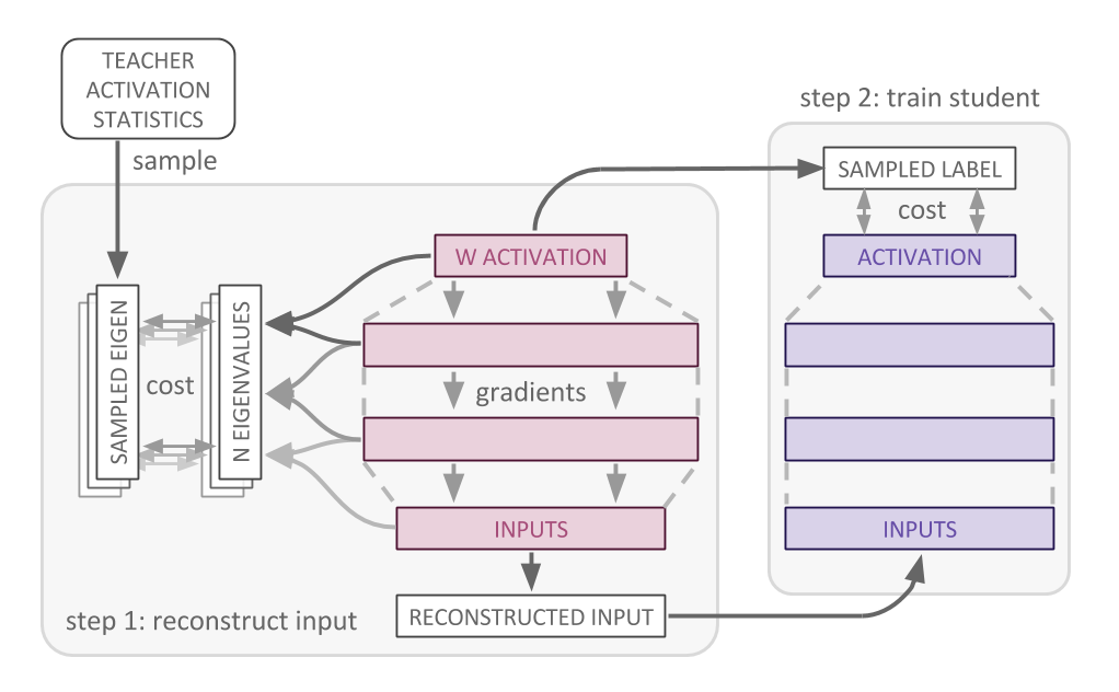
This is where the real magic happens. We use the saved metadata and the pre-trained model (but not the original dataset) to reconstruct/optimize a new dataset that maximally reconstruct samples from the activation statistics. These samples and the corresponding objective loss can take different forms (top_layer, all_layers, all_layers_dropout, spectral_all_layers, spectral_layer_pairs), which are discussed in the paper. Note that all_layers_dropout is meant for teacher models that are trained with dropout. Currently, we only provide hinton1200 that does. Also note that spectral optimization objectives require that the compute_graphwise_stats be set when running compute_stats

The pre-trained model is loaded, and a new graph is constructed using its saved weights, but as tf.constant. This ensures that the only thing being back-propagated to is the input tf.Variable, which is initialized to random noise.

The optimization_objective flag is needed to determine what loss to use (see paper for details, coming soon on arxiv). The dataset flag is only needed to determine io_size, so if you're using a pre-trained model+statistics that you don't have the original data for, you can mock the dataset class and simply provide the self.io_size attribute. Using all of this, a new dataset will be reconstructed and saved.

python main.py --run_name=experiment --model=hinton1200 --dataset=mnist \
    --procedure=optimize_dataset \
    --model_meta=summaries/experiment/train/checkpoint/hinton1200-8000.meta \
    --model_checkpoint=summaries/experiment/train/checkpoint/hinton1200-8000 \
    --optimization_objective=top_layer --lr=0.07
    # or all_layers, spectral_all_layers, spectral_layer_pairs

Distilling a Model Using One of the Reconstructed Datasets

You can then train a student network on the reconstructed dataset, and the temperature-scaled teacher model activations. This time, the dataset flag is the location where the reconstructed dataset was saved. Additionally, a student_model needs to be specified to be trained from scratch. If you want to evaluate the student's performance on the original test set (if you have access to it), you can specify it as the eval_dataset.

python main.py --run_name=experiment --model=hinton1200 \
    --dataset="summaries/experiment/data/data_optimized_top_layer_experiment_<clas>_<batch>.npy" \
    --procedure=distill \
    --model_meta=summaries/experiment/train/checkpoint/hinton1200-8000.meta \
    --model_checkpoint=summaries/experiment/train/checkpoint/hinton1200-8000 \
    --eval_dataset=mnist --student_model=hinton800 --epochs=30 --lr=0.00001

Distilling a Model Using Vanilla Knowledge Distillation

If you do have access to the original dataset, or you want to run Hinton's original Knowledge Distillation paper, you can just specify that dataset flag.

In order to run this baseline, you only need to have a pre-trained model, and the dataset it was originally trained with. This means you can skip the compute_stats and optimize_dataset steps.

python main.py --run_name=experiment --model=hinton1200 --dataset=mnist \
    --procedure=distill \
    --model_meta=summaries/experiment/train/checkpoint/hinton1200-8000.meta \
    --model_checkpoint=summaries/experiment/train/checkpoint/hinton1200-8000 \
    --eval_dataset=mnist --student_model=hinton800 --lr=0.0001

Tips and Tricks

When using the lenet models, it should be noted that the original paper specified that mnist was resized from 28x28 pixel images to 32x32. Thus, then using the convolutional models we provide, make sure to use the mnist_conv dataset, which automatically resize the input images. The rest of the usage should be exactly the same.

python main.py --run_name=experiment --model=lenet --dataset=mnist_conv \
    --procedure=train

python main.py --run_name=experiment --model=lenet --dataset=mnist_conv \
    --procedure=compute_stats \
    --model_meta=summaries/experiment/train/checkpoint/lenet-8000.meta \
    --model_checkpoint=summaries/experiment/train/checkpoint/lenet-8000

python main.py --run_name=experiment --model=lenet --dataset=mnist_conv \
    --procedure=optimize_dataset \
    --model_meta=summaries/experiment/train/checkpoint/lenet-8000.meta \
    --model_checkpoint=summaries/experiment/train/checkpoint/lenet-8000 \
    --optimization_objective=top_layer
    # or all_layers, spectral_all_layers, spectral_layer_pairs

python main.py --run_name=experiment --model=lenet \
    --dataset="summaries/experiment/data/data_optimized_top_layer_experiment_<clas>_<batch>.npy" \
    --procedure=distill \
    --model_meta=summaries/experiment/train/checkpoint/lenet-8000.meta \
    --model_checkpoint=summaries/experiment/train/checkpoint/lenet-8000 \
    --eval_dataset=mnist_conv --student_model=lenet_half --epochs=30

Visualization

The viz/ directory contains useful scripts you can run to visualize the saved statistics and optimized datasets.

Print top layer per class means and standard deviations

python viz/print_stats.py --run_name=experiment

Vizualize per-class and per-pixel means, as well as a randomly selected example of an optimized dataset.

Note that pixel_intensities_batch.py expects a single batch, so you have to add the specific batch you want to visualize. Since batches are saved separately, we no longer have a script to visualize all batches at once.

python viz/pixel_intensities_batch.py \
    --dataset=summaries/experiment/data/data_optimized_all_layers_dropout_experiment_0_0.npy

Per-class and per-pixel means and randoms image

Compare per-class, per-output normal distribution for both student and teacher.

Note that this requires that you have run compute_stats on a distilled student model. You might also want to play with the script to make each subplot zoomed in the best area (or apply a softmax over each mean/stddev pair of the statistics).

python viz/stats_viz.py \
    --teacher_stats=summaries/experiment/stats/activation_stats_experiment.npy \
    --student_stats=summaries/train_distilled_student/stats/activation_stats_train_distilled_student.npy

See what a sample from the top layer statistics looks like.

python viz/get_stats_sample.py --run_name=experiment

License

MIT

Appendix

For a longer description of each optimization objective, please refeer to the paper, which will be published on arxiv soon. In the meantime, if this readme was not sufficient, here are some diagrams from the paper:


Hinton's Knowledge Distillation

Top Layer Input Reconstruction and Distillation	All Layers Input Reconstruction and Distillation

Spectral All Layers Input Reconstruction and Distillation	Spectral Layer Pairs Input Reconstruction and Distillation