Trajectory Construction from Raw Data

Purpose

Data tells a story so let's find it!

Contained in the data below is all the information to reconstruct a fairly complex vehicle trajectory.

Raw Input Data

The data preprocessed from CSVs looks like this:

timestamp	displacement	yaw_rate	acceleration
0.0	0	0.0	0.0
0.25	0.0	0.0	19.6
0.5	1.225	0.0	19.6
0.75	3.675	0.0	19.6
1.0	7.35	0.0	19.6
1.25	12.25	0.0	0.0
1.5	17.15	-2.82901631903	0.0
1.75	22.05	-2.82901631903	0.0
2.0	26.95	-2.82901631903	0.0
2.25	31.85	-2.82901631903	0.0
2.5	36.75	-2.82901631903	0.0
2.75	41.65	-2.82901631903	0.0
3.0	46.55	-2.82901631903	0.0
3.25	51.45	-2.82901631903	0.0
3.5	56.35	-2.82901631903	0.0

This data is currently saved in a file called trajectory_example.pickle. It can be loaded using a helper function.

Each entry in data_list contains four fields. Those fields correspond to timestamp (seconds), displacement (meters), yaw_rate (rads / sec), and acceleration (m/s/s).

Data Explained

timestamp - Timestamps are all measured in seconds. The time between successive timestamps ($\Delta t$) will always be the same within a trajectory's data set (but not between data sets).

displacement - Displacement data from the odometer is in meters and gives the total distance traveled up to this point.

yaw_rate - Yaw rate is measured in radians per second with the convention that positive yaw corresponds to counter-clockwise rotation.

acceleration - Acceleration is measured in $\frac{m/s}{s}$ and is always in the direction of motion of the vehicle (forward).

After processing this exact data, it's possible to generate this plot of the vehicle's X and Y position:

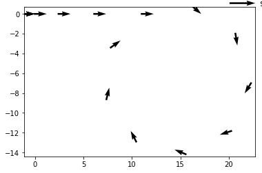
this vehicle first accelerates forwards and then turns right until it almost completes a full circle turn.

Making those cool arrows:

see demonstration code

Implementation

Take a processed data_list (with $N$ entries, each $\Delta t$ apart) as input:

get_speeds - returns a length $N$ list where entry $i$ contains the speed ($m/s$) of the vehicle at $t = i \times \Delta t$
get_headings - returns a length $N$ list where entry $i$ contains the heading (radians, $0 \leq \theta < 2\pi$) of the vehicle at $t = i \times \Delta t$
get_x_y - returns a length $N$ list where entry $i$ contains an (x, y) tuple corresponding to the $x$ and $y$ coordinates (meters) of the vehicle at $t = i \times \Delta t$
show_x_y - generates an x vs. y scatter plot of vehicle positions.

Initial Vehicle State