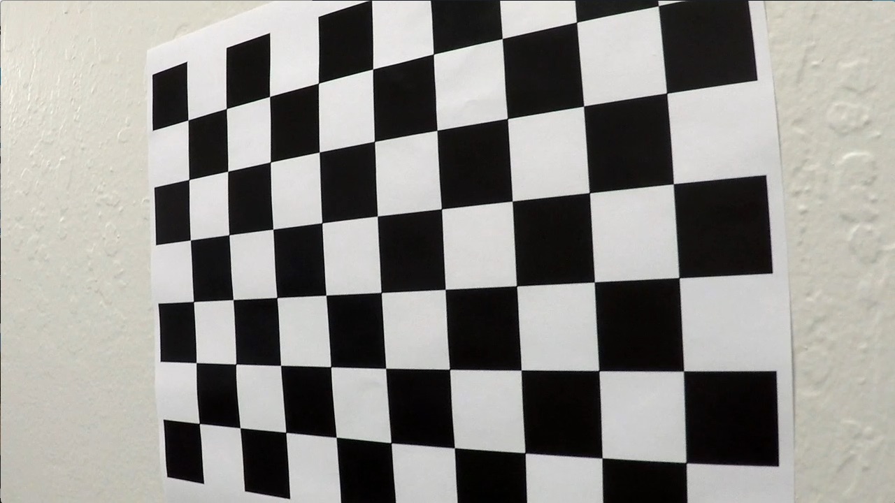
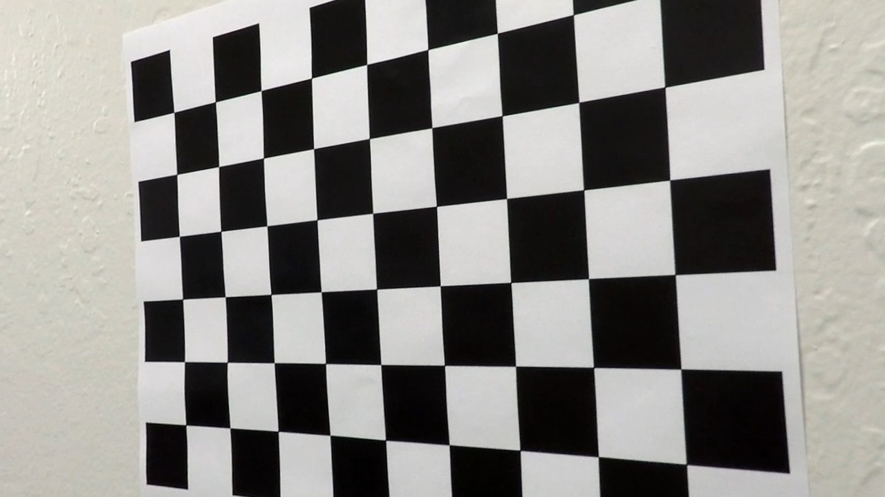
The code for the calculation of the distortion matrix of the camera can be found in the file ImageProcessor.py. When constructing an object of the class ImageProcessor the funciton calibrate_camerais called. This function checks whether the file camera_calibration_data.pickleis available which contains the camera_matrixand the camera_distortion_coefficients . If that is not the case, the function
compute_camera_calibration (ImageProcessor.py lines 29-58) is called, which computes the aforementioned camera_distortion_coefficients and camera_matrix using the provided calibration images and OpenCV's cv2.findChessboardCorners(gray, (9,6)) function. Afterwards the calibration data is stored in a pickle file for future use.
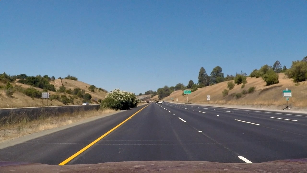
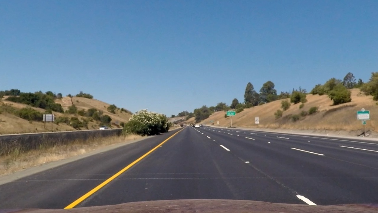
Below an example of an undistored image along with it's original, distorted counterpart is shown.
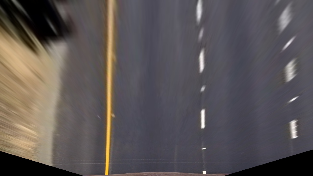
The next step is the computation of a transformation matrix to compute the perspective transform. Therefore, for points comprising a rectangle in the transformed image are needed. For this project, I used the following source and destination points to calculate the transformation and inverse transformation matrix.
| Source | Destination |
|---|---|
| 595, 450 | 440, 0 |
| 690, 450 | 840, 0 |
| 216, 720 | 440, 720 |
| 1115, 720 | 840, 720 |
The class ImageProcessor.py also handles the perspective transformation.
The code for this can be found in lines 85-10 in the file ImageProcessor.py. The transformation matrices are computed using the
cv2.getPerspectiveTransform function from OpenCV (cf. line 22 and 24 in ImageProcessor.py)
Below you can find an example image in original and transformed space, respectively.
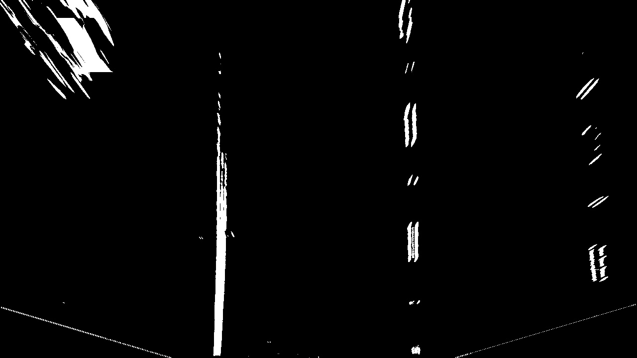
As discussed in the lecture, a combination of different binary thresholds is used to try to identify possible lane line pixels. In this project I used the following combination of thresholds:
- A [90,255] threshold on the s-channel of the image in hls color-space
- A [30,150] threshold on the x-gradient of the image computed using the sobel operator
- An or combination of the two thresholds above to obtain the final mask
The code for this masking operation can be found in
ImageProcessor.pyin lines 100-140. The pictures below shows an images to which this thresholding operation has been applied. Note that thresholding operation is performed on unwarped images, as this worked better.
Lane line detection and fitting a second order polynomial to the detected lane line pixels is implemented in class
LaneLine. An instance of this class is created for the detection of the left and the right lane line, respectively.
The LaneLine has a method called fit_lane_lane which takes in the warped, binary masked version of the image and an anchor point for the line computed by calculating a histogram of the lower half of the binary image.
There are two options for detecting the lane lines. The first is sliding window technique (lines 62-110 LaneLine.py)
The second option, that is used if the lane lines were successfully detected in the previous frame, is a faster approach
that searches for lane line pixels in the vicinity of the previous lane line (lines 110-130 LaneLine.py).
The faster option is always used if the lane lines were detected successfully in one of the previous five frames, other wise the slower sliding window technique is invoked.
Next, a second order polynomial is fitted to the detected lane line pixels. The coefficients of this polynomial are
then passed through a variant of a low-pass filter which takes into account the coefficients of the lane line polynomial from previous frames (lines 155-158 LaneLine.py)
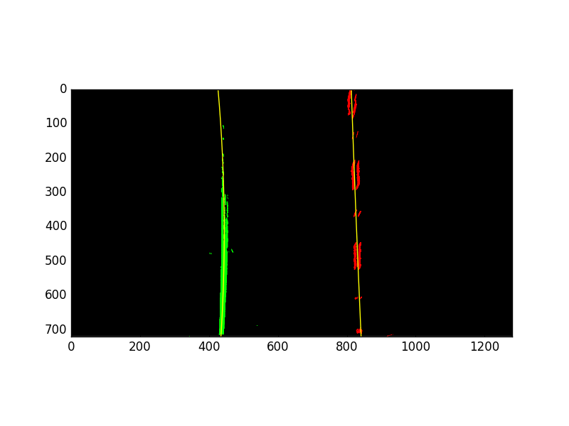
The figure below depicts the fitted polynomial in yellow.
Once the lane lines are detected, calculation of the lane line radii and position of the car is relatively straight forward.
However, the radii and position has to be calculated in meter not in pixels. The easiest way to ensure correct units is to
transform the lane line pixels into the real-world first, simply fit another polynomial to the data and then use standard calculus to compute the curvature (lines 160-170 LaneLine.py).
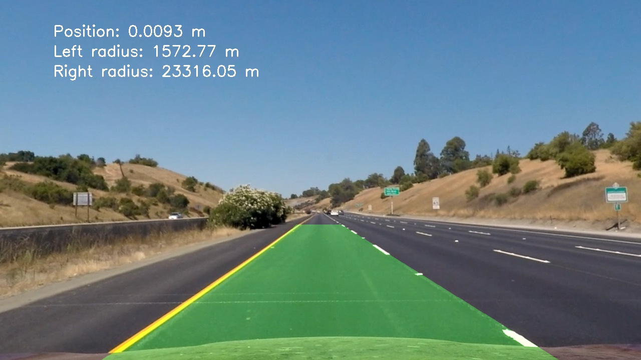
Applying the complete pipeline as described above, yields an annotated image where the detected lane area is marked in green and the radii of the left and right lane line are shown at the top, along with the deviation of the car from the center of the lane. An example image is shown below.
The project video can be found in this directory as output.mp4
After completing this project, I can see that a robust pipeline to detect lane line in a realistic setting is an immense challenge and significantly more difficult than I would have anticipated. Similar to the deep learning projects there are many many parameters which can be tuned. Having tested my pipeline on the harder challenge videos and seeing not so great performance there, I believe that major challenges for the current version of my pipeline are, amongst others:
- Quickly changing lighting conditions or shadows
- Changes in the color of the road surface
- Sharp curves
- Different lighting conditions due to weather conditions (cloudy, rainy,etc.)
- Different lighting condition at night
- Current implementation is too slow for real-time lane detection
There many things one could try to increase the robustness of the pipeline, some of these ideas can be found below:
- Further improve the binary masking of the images
- Introduce a preprocessing step and normalize the images
- Implement a sanity check if the detected lane lines are
- Use more advanced, non-parametric regression model instead of second order polynomial
- Use deep-learning instead of computer vision
