GAN-Supervised Dense Visual Alignment (GANgealing)
Official PyTorch Implementation of the CVPR 2022 Paper (Oral, Best Paper Finalist)
Paper | Project Page | Video | Two Minute Papers | Mixed Reality Playground 
This repo contains training, evaluation, and visualization code for the GANgealing algorithm from our GAN-Supervised Dense Visual Alignment paper. Please see our project page for high quality results.
GAN-Supervised Dense Visual Alignment
William Peebles, Jun-Yan Zhu, Richard Zhang, Antonio Torralba, Alexei Efros, Eli Shechtman
UC Berkeley, Carnegie Mellon University, Adobe Research, MIT CSAIL
CVPR 2022 - Oral, Best Paper Finalist
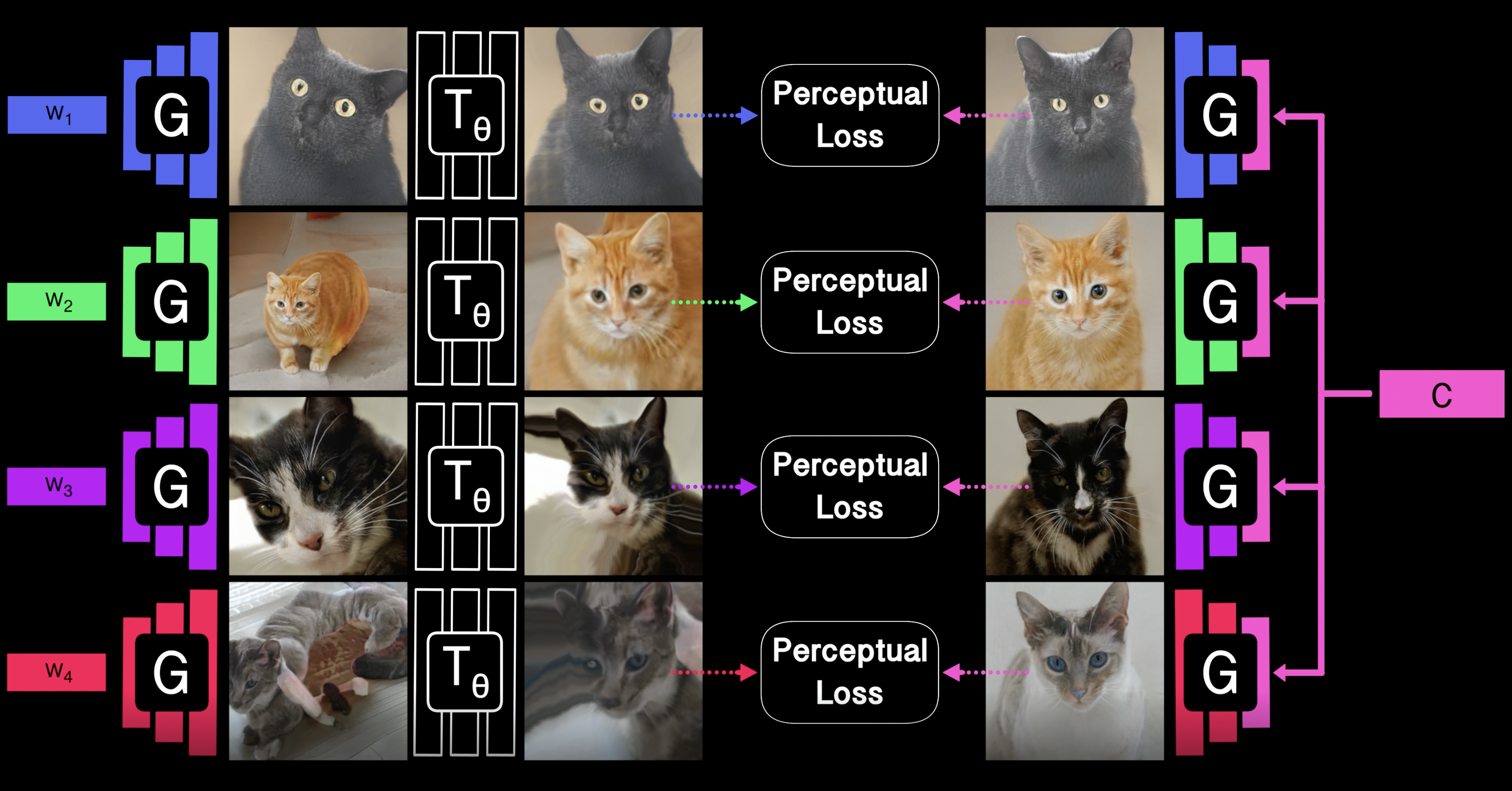
GAN-Supervised Learning is a method for learning discriminative models and their GAN-generated training data jointly end-to-end. We apply our framework to the dense visual alignment problem. Inspired by the classic Congealing method, our GANgealing algorithm trains a Spatial Transformer to warp random samples from a GAN trained on unaligned data to a common, jointly-learned target mode. The target mode is updated to make the Spatial Transformer's job "as easy as possible." The Spatial Transformer is trained exclusively on GAN images and generalizes to real images at test time automatically.
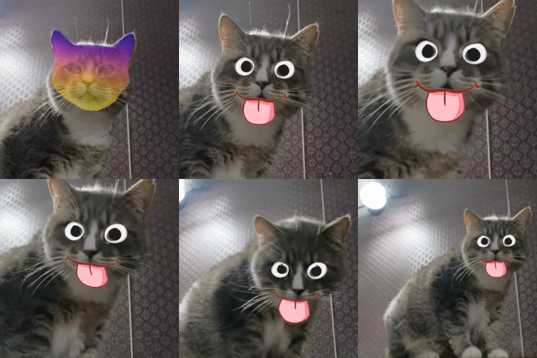
Once trained, the average aligned image is a template from which you can propagate anything. For example, by drawing cartoon eyes on our average congealed cat image, you can propagate them realistically to any video or image of a cat.
This repository contains:
- 🎱 Pre-trained GANgealing models for eight datasets, including both the Spatial Transformers and generators
- 💥 Training code which fully supports Distributed Data Parallel and the torchrun API
- 🎥 Scripts and a self-contained Colab notebook for running mixed reality with our Spatial Transformers
- ⚡ A lightning-fast CUDA implementation of splatting to generate high-quality warping visualizations
- 🚀 An implementation of anti-aliased grid sampling useful for Spatial Transformers (thanks Tim Brooks!)
- 🎆 Several additional evaluation and visualization scripts to reproduce results from our paper and website
First, download the repo and add it to your PYTHONPATH:
git clone https://github.com/wpeebles/gangealing.git
cd gangealing
export PYTHONPATH="${PYTHONPATH}:${PWD}"
We provide an environment.yml file that can be used to create a Conda environment:
conda env create -f environment.yml
conda activate gg
This will install PyTorch with a recent version of CUDA/cuDNN. To install CUDA 10.2/cuDNN 7.6.5 specifically, you can use environment_cu102.yml in the above command. See below for details on performance differences between CUDA/cuDNN versions.
If you use your own environment, you need a recent version of PyTorch (1.10.1+). Older versions of PyTorch will likely have problems building the StyleGAN2 extensions.
The applications directory contains several files for evaluating and visualizing pre-trained GANgealing models.
Using our Pre-trained Models: We provide several pre-trained GANgealing models: bicycle, cat, celeba, cub, dog and tvmonitor. We also have pre-trained checkpoints
for our car and horse clustering models. You can use any of these models by specifying them with the --ckpt argument; this will automatically download and cache
the weights. The relevant hyperparameters for running the model (most importantly, the --iters argument) will be automatically loaded as well. If you want to use your own test time hyperparameters, add --override to the command; see an example here.
The --output_resolution argument controls the size of congealed images output by the Spatial Transformer. For the highest quality results, we recommend setting this equal to the value you provide to --real_size (default value is 128).
We use LMDBs for storing data. You can use prepare_data.py to pre-process input datasets. Note that setting-up real data is not
required for training.
LSUN: The following command will automatically download and pre-process the first 10,000 images from LSUN Cats (you can change --lsun_category and --max_images):
python prepare_data.py --input_is_lmdb --lsun_category cat --out data/lsun_cats --size 512 --max_images 10000If you previously downloaded an LSUN LMDB yourself (e.g., at path_to_lsun_cats_download), you can instead use the following command:
python prepare_data.py --input_is_lmdb --path path_to_lsun_cats_download --out data/lsun_cats --size 512 --max_images 10000Image Folders: For any dataset where you have all images in a single folder, you can pre-process them with:
python prepare_data.py --path folder_of_images --out data/my_new_dataset --pad [center/border/zero] --size Swhere S is the square resolution of the resized images.
SPair-71K: You can download and prepare SPair for PCK evaluation (e.g., for Cats) with:
python prepare_data.py --spair_category cat --spair_split test --out data/spair_cats_test --size 256CUB: We closely follow the pre-processing steps used by ACSM for CUB PCK evaluation. You can download and prepare the CUB validation split with:
python prepare_data.py --cub_acsm --out data/cub_val --size 256vis_correspondence.py produces a video depicting real images being gradually aligned with our Spatial Transformer network.
It also can be used to visualize label/object propagation:
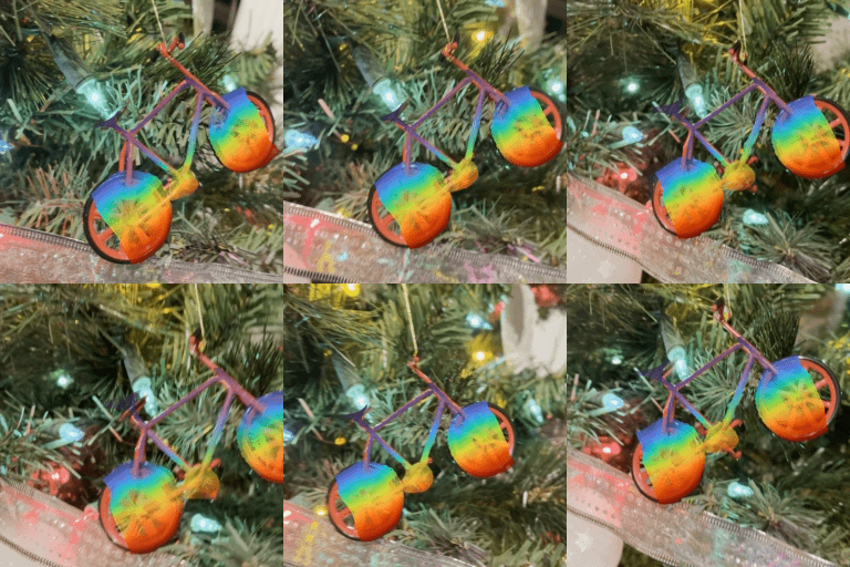
python applications/vis_correspondence.py --ckpt cat --real_data_path data/lsun_cats --vis_in_stages --real_size 512 --output_resolution 512 --resolution 256 --label_path assets/masks/cat_mask.png --dset_indices 2363 9750 7432 1946Dense Tracking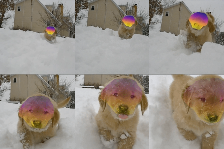 |
Object Propagation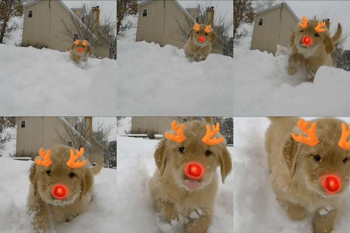 |
Congealed Video |
mixed_reality.py applies a pre-trained Spatial Transformer per-frame to an input video. We include several objects
and masks you can propagate in the assets folder.
The first step is to prepare the video dataset. If you have the video saved as an image folder (with filenames in order based on timestamp), you can run:
python prepare_data.py --path folder_of_frames --out data/my_video_dataset --pad center --size 1024This command will pre-process the images to square with center-cropping and resize them to 1024x1024 resolution.
You can specify --pad border to perform border padding instead of cropping or --pad resize_small_side to preserve aspect ratio. No matter what you choose for --pad, the value you use for --size needs to be a multiple of 128.
If your video is saved in mp4, mov, etc. format, we provide a script that will convert it into frames via FFmpeg:
./process_video.sh path_to_videoThis will save a folder of frames in the data/video_frames folder, which you can then run prepare_data.py on as described above.
Now we can run GANgealing on the video. For example, this will propagate a cartoon face via our LSUN Cats model:
torchrun --nproc_per_node=NUM_GPUS applications/mixed_reality.py --ckpt cat --objects --label_path assets/objects/cat/cat_cartoon.png --sigma 0.3 --opacity 1 --real_size 1024 --resolution 8192 --real_data_path path_to_my_video --no_flip_inferenceThis will efficiently parallelize the evaluation of the video over NUM_GPUS. Here is a quick overview of some arguments you can use with this script (see mixed_reality.py for all options):
--save_framescan be specified to significantly reduce GPU memory usage (at the cost of speed)--label_pathpoints to the RGBApngfile containing the object/mask you are propagating--objectswill propagate RGB values from yourlabel_pathimage. If you omit this argument, only the alpha channel of thelabel_pathimage will be used, and an RGB colorscale will be created (useful for visualizing tracking when propagating masks)--no_flip_inferencedisables flipping, which is recommended for models that do not benefit much from flipping (e.g.,cat,celeba,tvmonitor)--resolutioncontrols the number of pixels propagated. When usingmixed_reality.pyto propagate objects, we recommend making this value very large (e.g.,8192for a 1K resolution video)--blend_algcontrols the blending algorithm (alpha,laplacian, orlaplacian_light)--sigmacontrols the radius of splatted pixels--opacitycontrols the opacity of splatted pixels--save_correspondenceswill save a tensor of shape(num_frames, num_points, 2)containing predicted pixel correspondences in(x,y)format
To propagate your own custom object, you need to create a new RGBA image saved as a png. You can take the
pre-computed average congealed image for your model of interest (located in assets/averages) and load it
into an image editor like Photoshop. Then, overlay your custom object on the template and export the object as an RGBA png image.
Pass the png file to the --label_path argument like above.
We recommend saving the object at a high resolution for the highest quality results (e.g., 4K resolution or higher if you are propagating to a 1K resolution video).
propagate_to_images.py runs the Spatial Transformer on real images. It will save
the congealed (aligned) output images to disk. Basic usage:
python applications/propagate_to_images.py --ckpt cat --real_data_path data/lsun_cats --real_size 512 --dset_indices 1922 2363 8558 7401 9750 7432 2105 53 1946Edit Propagation: Add --label_path assets/objects/cat/cat_vr_headset.png --objects -s 0.3 -o 1 --resolution 4096 to propagate a VR headset to the cat images.
Dense Correspondence: Add --label_path assets/masks/cat_mask.png to propagate a mask.
Average Image: Add --n_mean 5200 to compute the average congealed image over 5200 input images. If you use this argument, you can call the script with torchrun --nproc_per_node NUM_GPUS instead of python to speed it up.
The main difference between this script and vis_correspondence.py is that this one just saves images instead of fancy video visualizations. It's much faster and takes less GPU memory as a result.
Our repo includes a fast implementation of PCK-Transfer in pck.py that supports multi-GPU evaluation. First, make sure you've set up either SPair-71K or CUB as described earlier. You can evaluate PCK-Transfer as follows:
To evaluate SPair-71K (e.g., cats category):
torchrun --nproc_per_node=NUM_GPUS applications/pck.py --ckpt cat --real_data_path data/spair_cats_test --real_size 256To evaluate CUB:
torchrun --nproc_per_node=NUM_GPUS applications/pck.py --ckpt cub --real_data_path data/cub_val --real_size 256 --num_pck_pairs 10000 --transfer_both_waysYou can also add the --vis_transfer argument to save a visualization of keypoint transfer.
Note that different methods compute PCK in slightly different ways depending on dataset. For CUB, the protocol used by past methods is to sample 10,000 random pairs from the validation set and evaluate bidirectional transfers. For SPair, fixed pairs are always used and the transfers are one-way. Our implementation of PCK supports both of these protocols to ensure accurate comparisons against baselines.
Finally, we also include a script that applies a pre-trained Spatial Transformer to align and filter an input dataset (e.g., for downstream GAN training): congeal_dataset.py
To use this, you will need two versions of your unaligned input dataset: (1) a pre-processed version (via prepare_data.py as described above), and (2) a raw, unprocessed version of the dataset stored in LMDB format. We'll explain how to create this second unprocessed copy below.
The first (pre-processed) dataset will be used to quickly compute flow scores in batch mode. The second (unprocessed) dataset will be fed into the Spatial Transformer to obtain the highest quality output images possible.
The first recommended step is to compute flow smoothness scores for each image in the dataset. As described in our paper, these scores do a good job at identifying (1) images the Spatial Transformer fails on and (2) images that are impossible to align to the learned target mode. The scores can be computed as follows:
torchrun --nproc_per_node=NUM_GPUS applications/flow_scores.py --ckpt cat --real_data_path my_dataset --real_size S --no_flip_inference, where my_dataset should be created with our prepare_data.py script as described above. This will cache a tensor of flow scores at my_dataset/flow_scores.pt.
Next is the alignment step. Create an LMDB of the raw, unprocessed images in your unaligned dataset using the --pad none argument:
python prepare_data.py --path folder_of_frames --out data/new_lmdb_data --pad none --size 0Finally, you can generate a new, aligned and filtered dataset:
torchrun --nproc_per_node=NUM_GPUS applications/congeal_dataset.py --ckpt cat --real_data_path data/new_lmdb_data --out data/my_new_aligned_dataset --real_size 0 --flow_scores my_dataset/flow_scores.pt --fraction_retained 0.25 --output_resolution O, where O is the desired output resolution of the aligned dataset and the --fraction_retained argument controls the percentage of images that will be retained based on flow scores. There are some other arguments you can adjust; see documentation in congeal_dataset.py for details.
Here's an example of loading and running our pre-trained unimodal Spatial Transformers to align an input image:
from models import get_stn
from utils.download import download_model, PRETRAINED_TEST_HYPERPARAMS
from utils.vis_tools.helpers import load_pil, save_image

model_class = 'cat'  # choose the class you want to use
resolution = 512  # resolution the input image will be resized to (can be any power of 2)
image_path = 'my_image.jpeg'  # path to image you want to align

input_img = load_pil(image_path, resolution)  # load, resize to (resolution, resolution) and normalize to [-1, 1]
ckpt = download_model(model_class)  # download model weights
stn = get_stn(['similarity', 'flow'], flow_size=128, supersize=resolution).to('cuda')  # instantiate STN
stn.load_state_dict(ckpt['t_ema'])  # load weights
test_kwargs = PRETRAINED_TEST_HYPERPARAMS[model_class]  # load test-time hyperparameters
aligned_img = stn.forward_with_flip(input_img, output_resolution=resolution, **test_kwargs)  # forward pass through the STN
save_image(aligned_img, 'output.png', normalize=True, range=(-1, 1))  # save to disk
If your input image isn't square you may want to pad or crop it beforehand. Also, stn supports batch mode, so input_img can be an (N, C, H, W) tensor containing multiple images, in which case aligned_image will also be (N, C, H, W).
The clustering models are usable in most places the unimodal models are (with a few current exceptions, such as flow_scores.py and congeal_dataset.py). To load the clustering models, add --num_heads K (we do this automatically if you're using one of our pre-trained models). There are also several files that let you propagate from a chosen cluster with the --cluster cluster_index argument (e.g., mixed_reality.py and vis_correspondence.py). Please refer to the documentation in those files for details.
We include several training scripts here. Running these scripts will automatically download pre-trained StyleGAN2 generator weights (included in our GANgealing checkpoints) and begin training. There are lots of training hyperparameters you can change; see the documentation here.
Training with Custom StyleGANs: If you would like to run GANgealing with a custom StyleGAN2(-ADA) checkpoint, convert it using the convert_weight.py script in the rosinality repository, and then pass it to --ckpt when calling train.py. If you're using an architecture other than the config-f StyleGAN2 (e.g., the auto config for StyleGAN2-ADA), make sure to specify values for --n_mlp, --dim_latent, --gen_channel_multiplier and --num_fp16_res so the correct generator architecture is instantiated.
Perceptual Loss: You can choose between two perceptual losses: LPIPS (--loss_fn lpips) or a self-supervised VGG pre-trained with SimCLR on ImageNet-1K (--loss_fn vgg_ssl). The weights will be automatically downloaded for both. Note that we recommend higher --tv_weight values when using lpips. We found 1000 to be a good default for vgg_ssl and 2500 a good default for lpips.
Clustering: When training a clustering model (--num_heads > 1), you will need to train a cluster classifier network afterwards to use the model on real images. This is done with train_cluster_classifier.py; you can find an example command here.
Note
For the majority of experiments in our paper, we trained using 8 GPUs and a per-GPU batch size of 5. If you train with fewer GPUs, you will likely need to increase your per-GPU batch size via the--batchargument in order to train models to high performance.
We have found on some GPUs that GANgealing training and inference runs faster at low batch sizes with CUDA 10.2/cuDNN 7.6.5 compared to CUDA 11/cuDNN 8. For example, on RTX 6000 GPUs with a per-GPU batch size of 5, training is 3x faster with CUDA 10.2/cuDNN 7.6.5. However, for high per-GPU batch sizes (32+), CUDA 11/cuDNN 8 seems to be faster. We have also observed very good performance with CUDA 11 on A100 GPUs using a per-GPU batch size of 5. We include two environments in this repo: environment.yml will install recent versions of CUDA/cuDNN whereas environment_cu102.yml will install CUDA 10.2/cuDNN 7.6.5. See here for more discussion.
If our code or models aided your research, please cite our paper:
@inproceedings{peebles2022gansupervised,
  title={GAN-Supervised Dense Visual Alignment},
  author={William Peebles and Jun-Yan Zhu and Richard Zhang and Antonio Torralba and Alexei Efros and Eli Shechtman},
  booktitle={CVPR},
  year={2022}
}We thank Tim Brooks for his anti-aliased sampling code and helpful discussions. We thank Tete Xiao, Ilija Radosavovic, Taesung Park, Assaf Shocher, Phillip Isola, Angjoo Kanazawa, Shubham Goel, Allan Jabri, Shubham Tulsiani, and Dave Epstein for helpful discussions. This material is based upon work supported by the National Science Foundation Graduate Research Fellowship Program under Grant No. DGE 2146752. Any opinions, findings, and conclusions or recommendations expressed in this material are those of the authors and do not necessarily reflect the views of the National Science Foundation. Additional funding provided by Berkeley DeepDrive, SAP and Adobe.
This repository is built on top of rosinality's excellent PyTorch re-implementation of StyleGAN2.

