Eddy covariance workflow

Overview

The eddy covariance (EC) workflow demonstrates how to use openeddy package together with REddyProc package to facilitate automated and reproducible EC data post-processing. The presented EC workflow is a set of post-processing steps that were applied for a particular cropland site CZ-KrP. The main purpose of EC workflow is to show how to utilize the software infrastructure. It is not meant to represent the optimal best post-processing workflow, especially concerning the quality control. The openeddy provides enough flexibility for users to adapt post-processing to specifics of their site and will hopefully facilitate discussion and exchange of best practices concerning various types of ecosystems and EC setups.

Comments in the workflow files explain how individual steps lead to the desired output. If you look for the settings and details about the openeddy functions, see openeddy documentation. Notice that there is also a set of interactive openeddy tutorials that provide more context.

Requirements

The EC workflow is currently aligned with EddyPro software output. It is expected that meteorological data passed its own separate workflow (not covered by openeddy) and are already converted to physical units and underwent quality control. Although KRP16 site-year example below contains already gap-filled meteorological data, gaps are allowed. Processing of multiple or incomplete years is supported but it requires edits in EC workflow scripts.

Adapting workflow for a new site mainly requires column renaming (variable names expected by used packages), preferably within EC workflow code (alternatively directly in input data). Support for other EC processing software (e.g. TK3, EdiRe, EddyUH, EddySoft) is not explicitly provided but alternative workflow should be achievable already with the existing openeddy capabilities. The easiest approach could be to remap_vars() using the pairing of column names of EddyPro full output and the EC processing software used. EddyPro-specific tests/filters mainly present in extract_QC() would need to be substituted for their alternatives. The KRP16 micrometeorological (meteo) data are formatted in a specific way that is handled by specialized function read_MeteoDBS(). To achieve similar results, you can use read_eddy() in combination with merge_eddy() to read and validate general data frame with meteo data.

In order to run fetch_filter(), QC workflow also requires the region of interest (ROI) outline for given site-year. ROI is provided by the user in a form of numeric vector (see ROI boundary section below and https://github.com/lsigut/ROI_boundary).

Usage

To run EC workflow for the example site-year KRP16:

Download KRP16 - before processing.zip from Zenodo and unzip. Run workflow files in specified order according to instructions there:

data_preparation workflow: formatting and merging inputs.
QC workflow: eddy covariance quality control.
GF_&_FP workflow: uStar-filtering, gap-filling and flux partitioning.
Summary workflow: aggregation and summary of results.

All workflows should be first adapted to given site-year properties and commands run one by one, following the included instructions suggesting edits when needed. The workflow files are structured so that mostly only the upper sections require user inputs while the remainder is mostly automated.

Note that sourcing the QC workflow will not produce desired outcome if variable interactive = TRUE because interactive functions are included. Once the manual QC is finalized and automatically saved, changing to interactive = FALSE allows to reproduce all results by sourcing all workflows.

You can compare your results with those of KRP16 - processed.zip at Zenodo. Notice that in order to obtain identical results, you would need to copy the subjective manual screening done by site PI located at ./Level 2/Quality checking/KRP16_manual_QC.csv.

Description

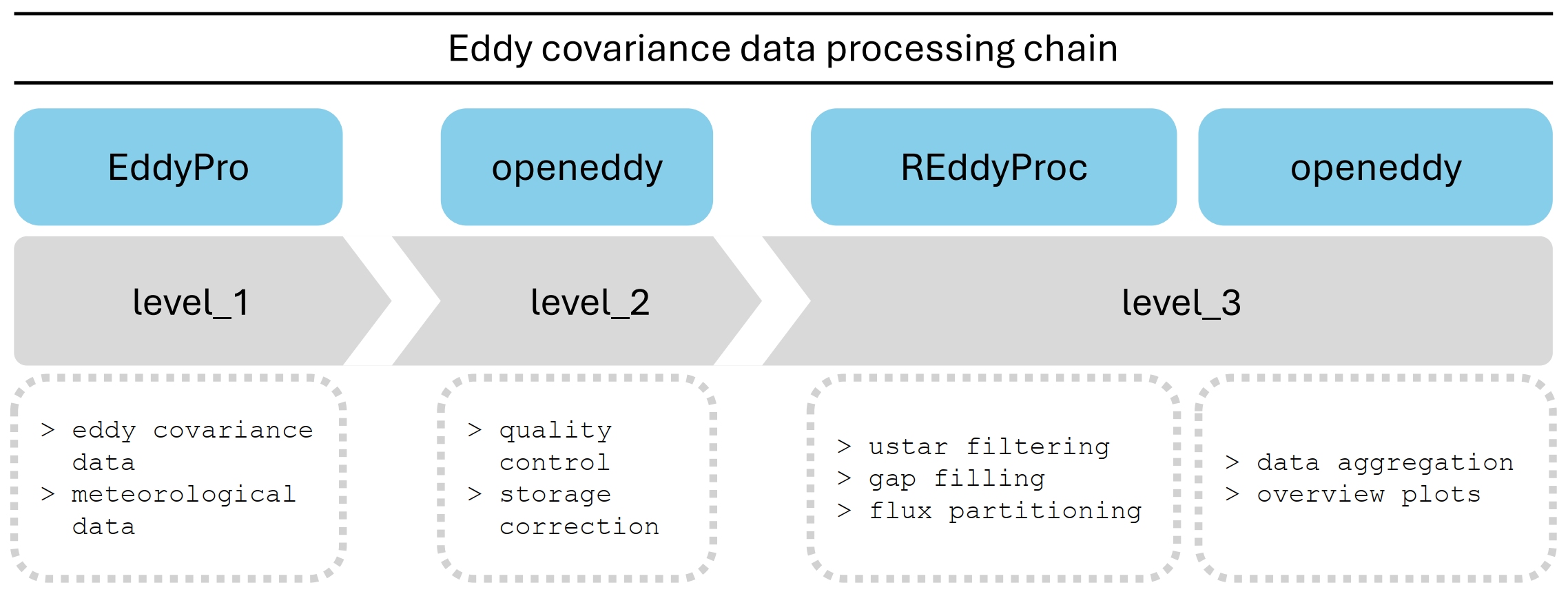
The proposed workflow allows to process eddy covariance data with single processing chain consisting of four stages:

Storage: estimate storage flux to allow for storage correction. Computation of storage flux from profile measurements is currently not available. EddyPro full output provides storage fluxes computed by discrete (one point) approach. While this is sufficient for sites with short canopy (e.g. the example cropland site CZ-KrP), one point approximation is less suitable with increasing EC measurement height. Implementation of profile measurements for computation of storage flux is outside of scope of openeddy package.
Quality control (QC): load the EddyPro output and gap-filled meteorological data and apply automated tests and filters implemented in openeddy to quality check fluxes of momentum (Tau), sensible (H) and latent heat (LE) and net ecosystem exchange (NEE). Export documentation of applied QC and produce the outputs needed in next steps. QC workflow produces files at .\Level 2\Quality checking\ and .\Level 2\Input for gap-filling\ folders.
Gap-filling and flux partitioning (GF & FP): combine utilities of REddyProc and openeddy to gap-fill (H, LE, NEE), partition (NEE) and visualize (H, LE, NEE) fluxes. The setup allows to change and document some processing options in an organized way. Computation of bootstrapped friction velocity threshold is included. GF & FP workflow produces files at .\Level 3\Gap-filling\REddyProc\.
Summary: visualize processed data, convert units and aggregate results to daily, weekly, monthly and yearly timescales. A limited amount of computed parameters is also produced, including different uncertainty estimates. Summary workflow produces files at .\Level 3\Summary\REddyProc\.

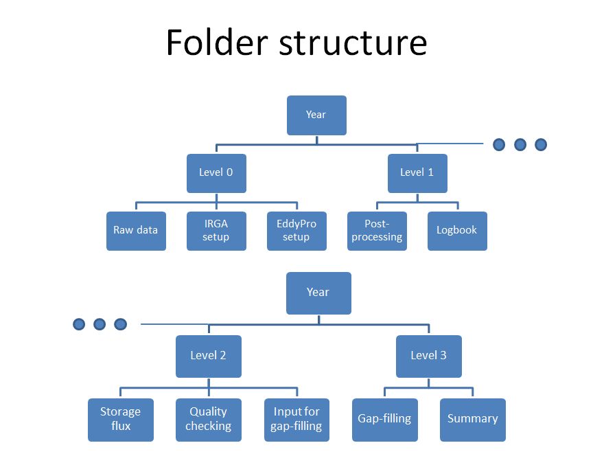
The EC workflow assumes certain folder structure that makes data handling more effective. The folder structure can be created using structure_eddy().

Level 0: raw data, related metadata and configuration files.
Level 1: half-hourly data processed by EddyPro and gap-filled meteorological data.
Level 2: results and documentation of QC, storage corrected fluxes for GF & FP.
Level 3: results of GF & FP and the dataset summaries.

The complete processing chain in the context of above folder structure can be summarized as:

ROI boundary

The outline delimiting the spatial extent of the studied ecosystem (region of interest; ROI) is specified by its ROI boundary that describes the distance from EC tower to the edge of the studied ecosystem for given wind direction. In order to work with openeddy, ROI boundary has to be provided as a numeric vector with following properties:

The number of circular sectors is the same as the number of provided distances (length of the vector).
The angular resolution of the ROI boundary is given by 360° / number of angular sectors.
The ROI boundary distances are assigned to the centers of their respective circular sectors with first sector centered on 0°.

ROI boundary example

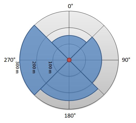
In this simplified case ROI boundary would be specified as:

c(150, 200, 250, 300)

Interpretation:

There would be 4 circular sectors with 90° angular resolution.
ROI boundary is specified for the whole first sector (315°, 45°] at the distance 150 m from tower (center of the sector is 0°).
Boundary of the second sector (45°, 135°] is at the distance 200 m.
Third sector (135°, 225°] is at the distance 250 m.
Fourth sector (225°, 315°] is at the distance 300 m.

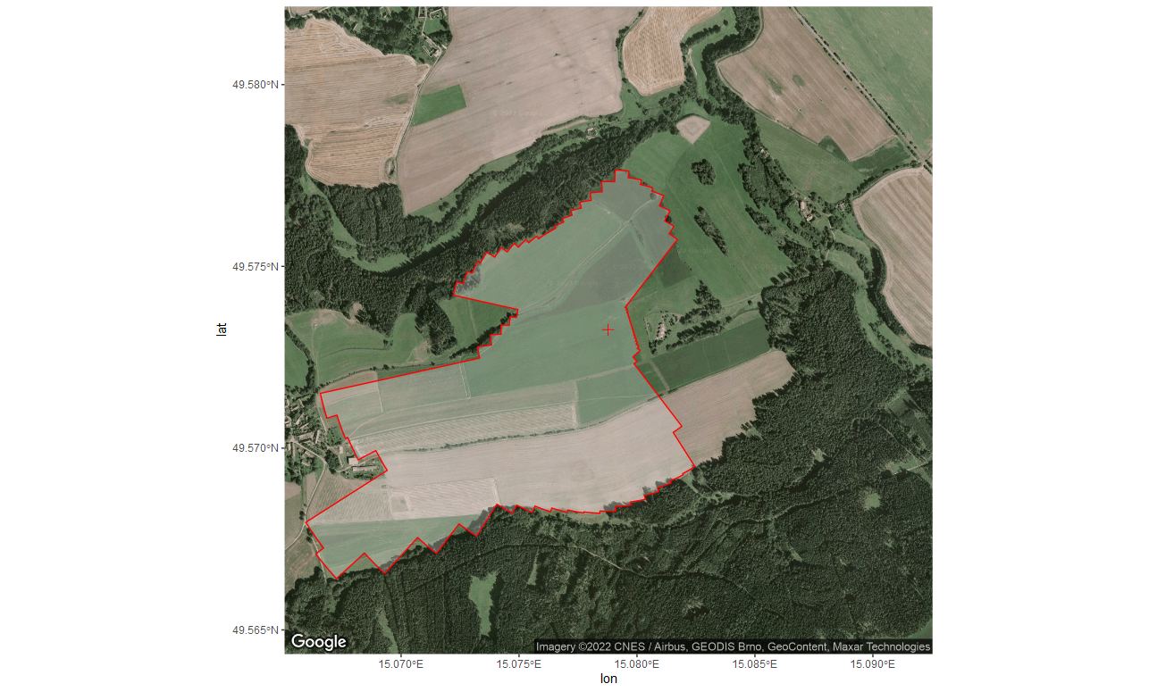
Realistic representation of ROI boundary can look e.g. like this:

Naming strategy with the EC workflow

In order to take advantage of openeddy default arguments, certain naming strategy is recommended.

EddyPro full output variable names are used with a few modifications if symbols were included in the variable name (e.g. Monin-Obukhov stability parameter (z-d)/L is corrected to zeta).

Expected names of meteorological variables are due to historical reasons:

GR: global radiation [W m-2]
PAR: photosynthetically active radiation [umol m-2 s-1]
Rn: net radiation [W m-2]
Tair: air temperature at EC height [degC]
Tsoil: soil temperature at soil surface [degC]
RH: relative humidity at EC height [%]
VPD: vapor pressure deficit at EC height [hPa]
P: precipitation [mm]

openeddy offers full flexibility concerning QC column names. However, in order to avoid QC column duplication and to partly document the type of QC test/filter and flux that it corresponds to, following naming strategy was devised:

QC prefixes

They specify which flux is affected by given QC column:

qc_Tau_, qc_H, qc_LE, qc_NEE: only applicable for the respective fluxes.
qc_SA_: applicable to fluxes relying only on sonic (Tau, H).
qc_GA_: applicable to fluxes relying on GA (LE, NEE); only GA issues considered.
qc_SAGA_: applicable to fluxes relying both on SA and GA (LE, NEE); both SA and GA issues considered.
qc_ALL_: applicable to all fluxes (in practice often not applied to Tau).

QC suffixes

They specify which QC test/filter was applied to get the QC flags:

_SSITC: steady state test and test of integral turbulence characteristics.
_spikesHF: check of high frequency data spike percentage in averaging period against thresholds.
_ampres: check of amplitude resolution in the recorded data.
_dropout: check of drop-outs, i.e. situations when the time series stays for “too long” on a value that is far from the mean.
_abslim: check of absolute limits when raw data are out of plausible range.
_skewkurt_sf, _skewkurt_hf, _skewkurt: check of skewness and kurtosis limits.
_discont_sf, _discont_hf, _discont: check of discontinuities that lead to semi-permanent changes in the time series.
_timelag_sf, _timelag_hf, _timelag: check of estimated timelags compared to the expected timelags.
_attangle: check of angle of attack.
_nonsteady: check of steadiness of horizontal wind.
_missfrac: check of missing data in averaging period against thresholds.
_scf: check of spectral correction factor against thresholds.
_wresid: check of mean unrotated w (double rotation) or w residual (planar fit) against thresholds.
_runs: check of runs with repeating values.
_lowcov: check of fluxes too close to zero (assuming issues during covariance computation).
_var: check of variances against thresholds.
_LI7200: check of CO2 and H2O signal strength against thresholds.
_interdep: flux interdependency.
_man: manual quality control.
_spikesLF: identification of likely outliers in low frequency data.
_fetch70: check of distance corresponding to 70% signal contribution against fetch distance for given wind direction.
_forGF: the composite QC column used to screen fluxes for gap-filling combining selected above test/filter results.

For details see documentation of extract_QC().

REddyProc naming strategy is available at MPI Online Tool website.

Manual QC guide

Theoretically, manual QC is introducing subjectivity to the workflow and should be avoided. However, in practice, certain events can occur that might be difficult to screen based on auxiliary data or the tests are not sensitive enough to capture them. It should be noted that data not falling within the expected range might represent interesting rare phenomena and should be carefully investigated before manual removal. The screening typically depends on the user experience with the site, considering meteo conditions and phenology. Examples of manually excluded half-hours could be those affected by precipitation, strong advection and unexpected technical issues. Neighbors of outlying values or isolated points can be good candidates for exclusion as they might have escaped the automated screening. Change of weather fronts can lead to unexpected energy fluxes that however reflect real conditions. In these conditions it could depend on the research question whether such cases should be excluded.

Abbreviations

EC: Eddy Covariance
QC: Quality Control
SA: Sonic Anemometer
GA: Gas Analyzer
Tau: Momentum flux [kg m-1 s-2]
H: Sensible heat flux [W m-2]
LE: Latent heat flux [W m-2]
NEE: Net ecosystem exchange [umol m-2 s-1]
u: Longitudinal wind speed component [m s-1]
w: Vertical wind speed component [m s-1]
ts: Sonic temperature [degC]
h2o: H2O concentration [mmol mol-1]
co2: CO2 concentration [umol mol-1]

References

Publication describing openeddy is not yet available. When describing the proposed quality control scheme, please refer to:

McGloin, R., Sigut, L., Havrankova, K., Dusek, J., Pavelka, M., Sedlak, P., 2018. Energy balance closure at a variety of ecosystems in Central Europe with contrasting topographies. Agric. For. Meteorol. 248, 418-431. https://doi.org/10.1016/j.agrformet.2017.10.003

Other references relevant to the applied quality control:

Foken, T., Wichura, B., 1996. Tools for quality assessment of surface-based flux measurements. Agric. For. Meteorol. 78, 83–105. https://doi.org/10.1016/0168-1923(95)02248-1

Vickers, D. and Mahrt, L., 1997. Quality Control and Flux Sampling Problems for Tower and Aircraft Data. Journal of Atmospheric and Oceanic Technology, 14(3), 512-526. https://doi.org/10.1175/1520-0426(1997)014<0512:QCAFSP>2.0.CO;2

Mauder, M., Cuntz, M., Drüe, C., Graf, A., Rebmann, C., Schmid, H.P., Schmidt, M., Steinbrecher, R., 2013. A strategy for quality and uncertainty assessment of long-term eddy-covariance measurements. Agric. For. Meteorol. 169, 122-135, https://doi.org/10.1016/j.agrformet.2012.09.006

The methodology and benchmark of REddyProc 1.1.3 is described in the following paper:

Wutzler, T., Lucas-Moffat, A., Migliavacca, M., Knauer, J., Sickel, K., Šigut, L., Menzer, O., and Reichstein, M. (2018): Basic and extensible post-processing of eddy covariance flux data with REddyProc, Biogeosciences, 15, 5015-5030, https://doi.org/10.5194/bg-15-5015-2018.

lsigut/EC_workflow