Python unfolding implementation based on:
- Barlow, Beesten: Fitting using finite Monte Carlo samples (1993)
- Blobel: An unfolding method for high energy physics experiments (2002)
Data for building the response matrix and testing the unfolding is generated by the mc_data_gen class. The generated data is the same as used by Blobel in his examples.
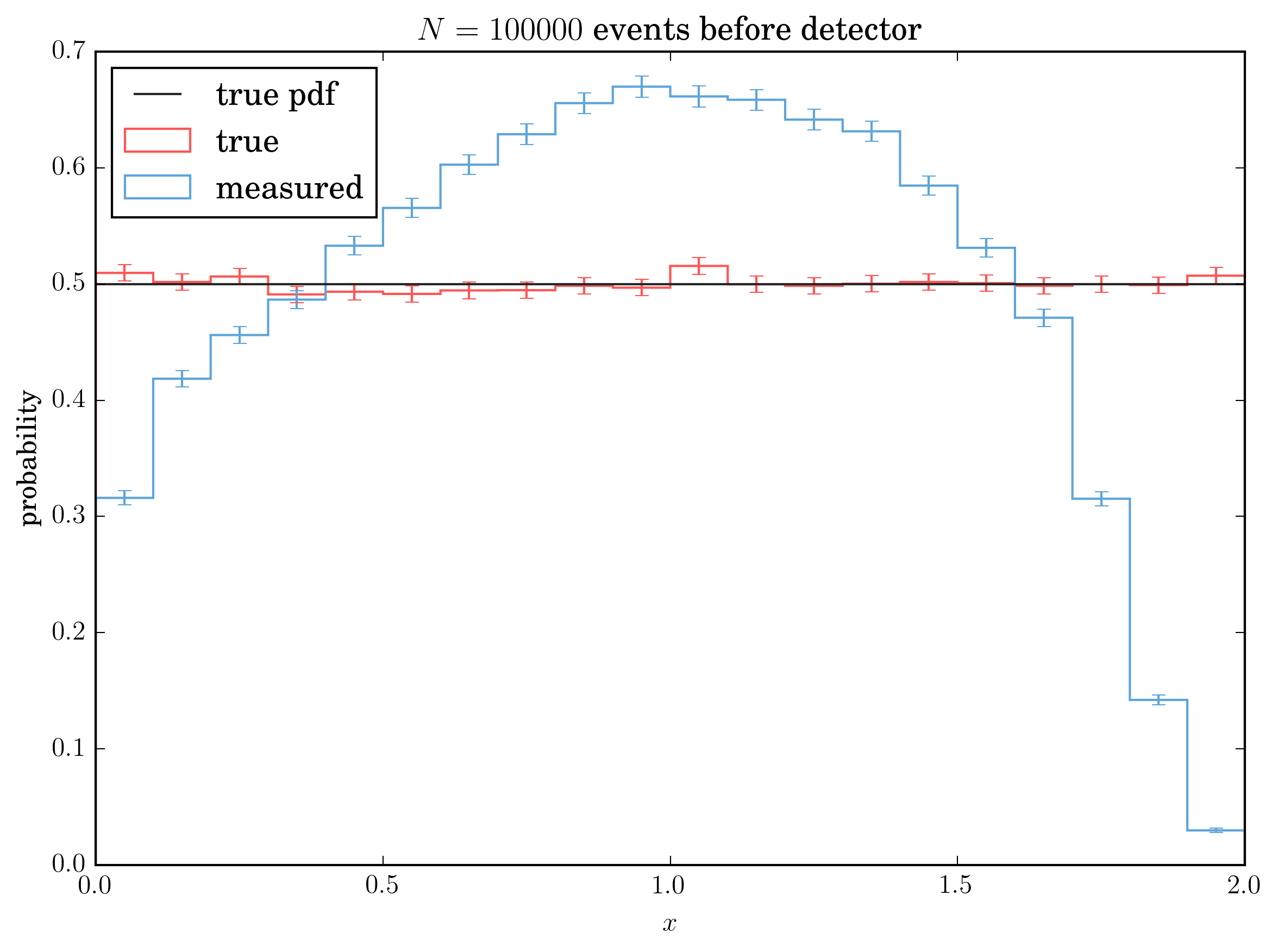
The model is trained (the response matrix is build) with a flat spectrum, which is simply generated from a uniform distribution $$ f_{MC} = \frac{1}{x_h - x_l} $$
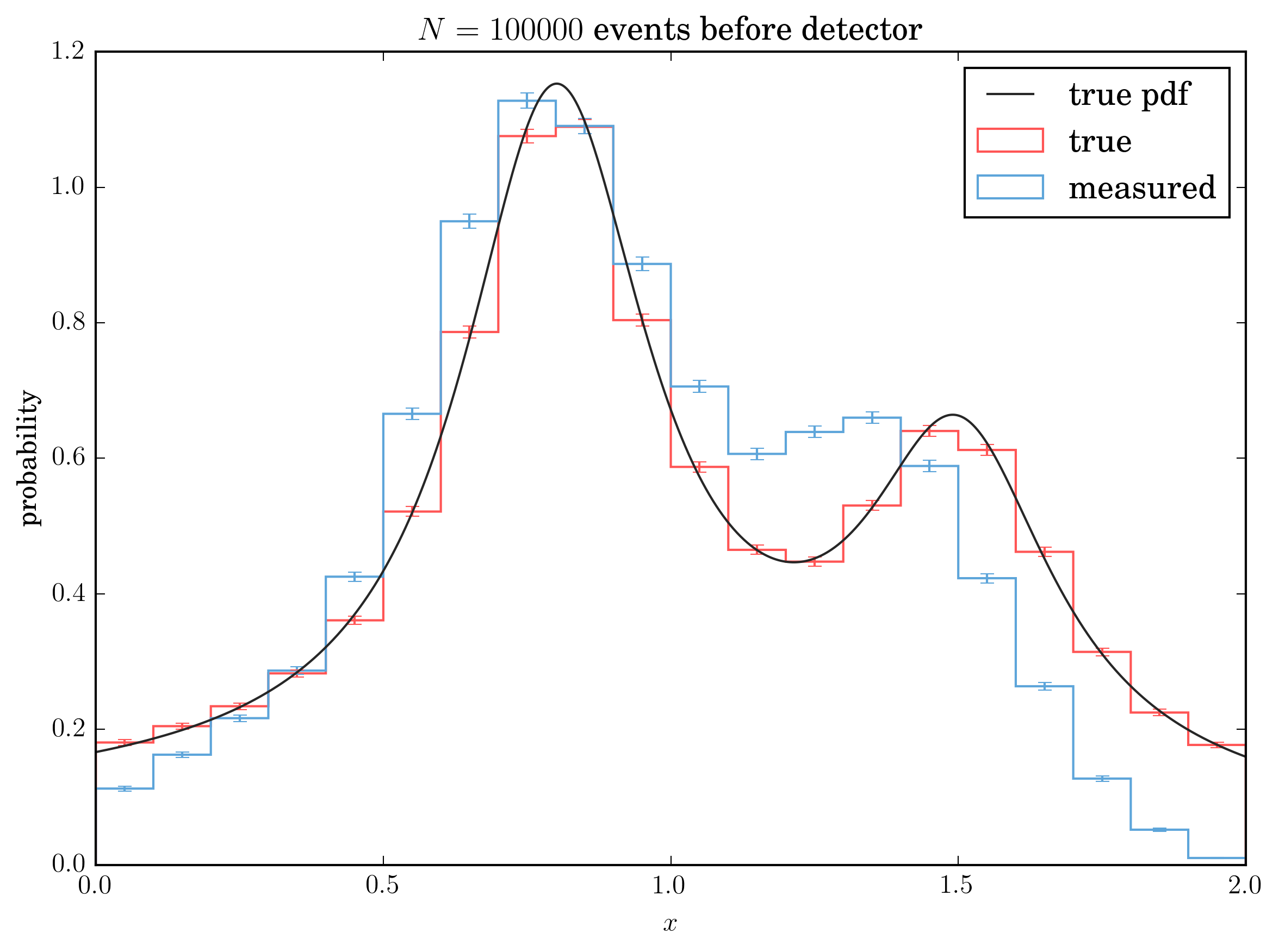
For the actual unfolding part a triple lorentzian is used. The pdf of the true distribution is the sum of three lorentz function normed correctly to unity: $$ f_\text{true} = \sum_{i=1}^{3} b_k \frac{g_k^2}{(x-x_k^2) + g_k^2} $$
with the parameters
| k | b_k | x_k | g_k |
|---|---|---|---|
| 1 | 1 | 0.4 | 2.0 |
| 2 | 10 | 0.8 | 0.2 |
| 2 | 5 | 1.5 | 0.2 |
The normalization in the interval
The measured distribution is obtained from the true one by applying a limited acceptance probability, a systematic shift and a gaussian smearing. For the standard example, the acceptance probability is $$ p_\text{acc} = 1 - \frac{(x - 1)^2}{2} $$
Not accepted events have weight values of 0. The function $$ y_\text{shift} = x - \frac{x}{20} $$
shifts the data. The smearing is applied with a standard normal distribution with
Example of both distribution with 10000 generated numbers is shown below, with the true distribution and after detector effects have been applied.

