This study proposes an algorithmic method to seamlessly blend two photos together into a single, natural looking rendering. Typically, this process is complete manually via a photo editing software such as photoshop and may take tens of minutes to hours to complete depending on the size and accuracy of the final image required. With this method, we can achieve similar, if not superior results within a fraction of the time.
The aim of this study is to use image processing techniques to autonomously and efficiently identify and cutout a source image, copy it to a specific location of a target image, modify the source image so that the indices of pixels in the source image and target image correspond, and output a natural looking and seamlessly blended image.
An expanded description of this model implimentation can be found on its project page here:
https://www.michaelhasey.com/gradient-domain-fusion
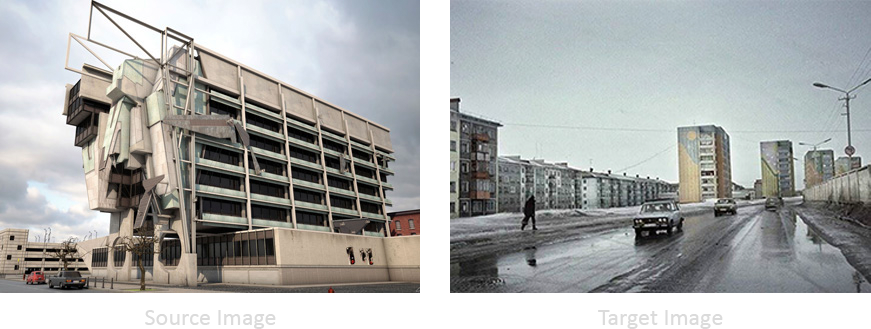
The dataset used includes a series of source and target image pairs in jpg format. The source image represents the image that will be cut out, pasted and blended into the target image.
An example image pair has been included and can be found here:
data/source_01.jpg
data/target_01.jpg
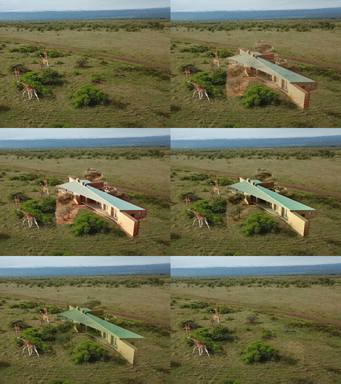
To begin, users must select a source image and a target image. The source image will be the one in which content is copied from, and the target image is the one in which that content will be “pasted” into. As the algorithm does not modify perspective, images with similar vantage points and perspectives work best. Finally, similar matching backgrounds between the source and target image, for example the savannah grasslands shown here, helps to ensure a cohesive final image.
A masking algorithm is used to define the source and target regions to blend. A graphic user interface allows the user to first select the content in the source image to copy, then change its size and orientation, and finally define where it will be pasted into the target image. The resultant output is a newly defined source image with the source image content moved to the corresponding x-y orientation that matches its position in the target image as defined by the user, as well as a mask image which highlights the source image pixel area to be copied.
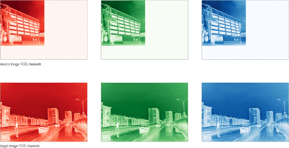
In order to move forward, both the target and source image must be split into their three individual RGB channel components (red, green, blue). This will allow us to colour match each individual source channel to its corresponding target channel. For example, colour matching the source image red channel to the target image red channel. A false color filter has been added to the images below to better illustrate the specific RGB channel associated to each image.
An image can be described as a series of x-y gradients, or relationships between each one of its individual pixels and their surrounding pixel neighbours in the x and y direction. As each image pixel can be represented by a number, its relationship to its neighbour can be described by the difference between their pixel values. For example, the gradient between a red pixel with value of 10 and a neighbouring blue pixel with a value of 4 is 6, or 10 - 4 = 6. This difference is called the derivative. By calculating and recording the derivatives of each pixel within the entire image, we can thus calculate the overall gradient of an image. With an RGB colour image, we first need to separate the image into its 3 channels before calculating the gradient. In the next step, we compare this gradient to the target or background image gradient in which it is being copied into and adjust each pixel in order for it to blend in colour and intensity.
Two matrices must be created in order to store numerical image gradients as well as their corresponding x,y positions within the image. This is also done so the original image can be recovered or rebuilt from this information. The first matrix is a sparse matrix where each line represents an individual pixel and its relationship to a single one of its 4 neighbours. Thus, the number of rows is equal to 4X the number of pixels in the source image being copied. The number of columns is equal to the number of pixels in the source image being copied. The second matrix is a 1 dimensional array that represents the known derivative or difference between a single pixel and one of its four neighbours. Hence the number of elements in this1d array is equal to 4X the number of source image pixels being copied. We can combine these two matrices together with a linear solver in order to recover the original image.
The previous step described how we can determine an images gradient, encode them into matrices, then convert them back into an image using a linear solver. In this next step, we take a similar approach but integrate the target image’s gradient as well in order to achieve the blend effect.
In order to do this, we use the Poisson Blending technique which is shown below. To summarize, the Poisson Blending technique reconstructs the source image gradient in a way that alters its pixel values while maintaining its overall gradient “shape”. Shape in this instance means the overall gradient pattern as illustrated in Step 4 above. By maintaining shape, the source image content, such as geometry and pattern, are maintained rather than distorted.
However, the Poisson Blending technique takes into account the colour of the target pixels that surrounding the source image and adjusts the source image pixels to match while maintaining content. Such pixel level modification is achieved by solving a “least squares” problem which aims to minimizes source image content distortion as much as possible while maximizing the colour cohesion between the source image pixels and neighbouring target image pixels. The power of this technique lies in its ability to modify pixels at an individual rather than universal level, thus leading to seamlessly blended images.
To run the code and blend a target and source image together, follow these steps.
1.Launch "masking_code.py" from terminal to create required images / mask needed for step 2.
masking_code.py
- specify source region to copy
- specify target region to paste into
- new target mask image created & saved in home directory
- new source image created & saved in home directory
- Run "Part_1.2_Poisson_Blending.ipynb" Jupyter Notebook with output being the final blended image.
Part_1.2_Poisson_Blending.ipynb
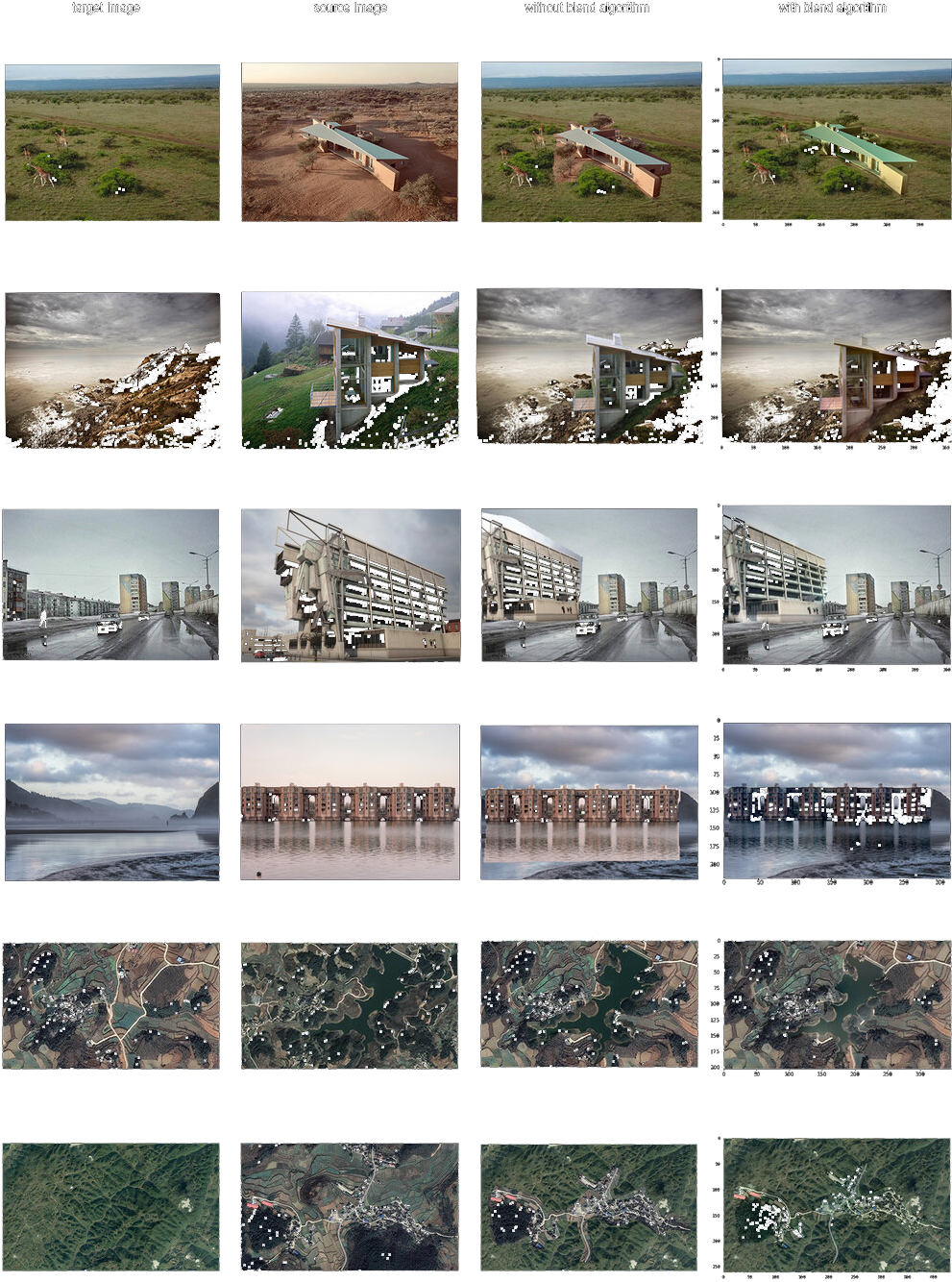
The below source and target image pairs were all blended using the above described Poisson Blending Technique.
This project was completed as part of Carnegie Melon University's Learning Based Image Synthesis course 16 726 taught by Jun-Yan Zhu in Spring of 2021.
If you find this project useful in your research, please consider citing:
@misc{mhasey2021,
    title={Image Blending Tool},
    author={Michael Hasey},
    year={2021},
}


