ThreeBodyDecay

Note

soon DEPRICATED

use ThreeBodyDecays.jl

that is going to be a registered package shortly

A framework for the amplitude analysis of multibody decay chains. The main focus of the project is the three-body decay and reactions required the Dalitz Plot analysis. The latter includes reactions with more then three particles, which however can be factorized to a product of sequential decays with $≤3$ products due to the lifetime of the long-lived particles. All particles can have arbitrary spin.

The framework is based on the publication, "Dalitz-plot decomposition for three-body decays" by JPAC Collaboration (M Mikhasenko at al.) (arxiv). The code inherits notations of the paper:

Particles are numbered 1,2,3, and 0 for the decay products and the mother particle, respectively.
s is a total invariant mass of three particles,
σ is a two-particle invariant mass squared, σₖ = (pᵢ+pⱼ)²,
θᵢⱼ is a scattering angle, an angle between vec pᵢ and - vec pₖ.
hat θₖ₍ⱼ₎ is a isobar angle (the Wigner angle of the 0-particle), an angle of vec pⱼ+pⱼ with respect the the chain j.
ζᵏᵢ₍₀₎ is the Wigner angle for the final-state particle (see the paper for the definition).

API for describing the decay

A type ThreeBodySystem is used to keep information of the three-body system (masses, spins, and parities). The DecayChain structure contain information on the spin of the intermediate resonance, its lineshape and $LS$ Clebsch-Gordan coefficient in the production and decay vertices.

Here is an example for amplitude description for Λb ⟶ Jψ p K, the reaction where the pentaquarks candidates were observed for the first time.

using ThreeBodyDecay # import the module
#
# decay Λb ⟶ Jψ p K
ms = (Jψ = 3.09, p=0.938, K = 0.49367, Lb = 5.62) # masses of the particles
# create two-body system
tbs = ThreeBodySystem(ms.Jψ, ms.p, ms.K; m0=ms.Lb,   # masses m1,m2,m3,m0
            two_js=ThreeBodySpins(2, 1, 0; two_h0=1])) # twice spin
Concerving = ThreeBodyParities('-',  '+',  '-'; P0='+')
Violating  = ThreeBodyParities('-',  '+',  '-'; P0='-')

ThreeBodySystem creates an immutable structure that describes the setup. Two work with particles with non-integer spin, the doubled quantum numbers are stored.

The following code creates six possible decay channels. The lineshape of the isobar is specified by the second argument, it is a simple Breit-Wigner function in the example below.

# chains-1, i.e. (2+3): Λs with the lowest ls, LS
Λ1520  = DecayChainLS(1, σ->BW(σ, 1.5195, 0.0156); two_s = 3/2|>x2, parity = '+', Ps=Concerving, tbs=tbs)
Λ1690  = DecayChainLS(1, σ->BW(σ, 1.685,  0.050 ); two_s = 1/2|>x2, parity = '+', Ps=Concerving, tbs=tbs)
Λ1810  = DecayChainLS(1, σ->BW(σ, 1.80,   0.090 ); two_s = 5/2|>x2, parity = '+', Ps=Concerving, tbs=tbs)
Λs = (Λ1520,Λ1690,Λ1810)
#
# chains-3, i.e. (1+2): Pentaquarks with the lowest ls, LS
Pc4312 = DecayChainLS(3, σ->BW(σ, 4.312, 0.015); two_s = 1/2|>x2, parity = '+', Ps=Concerving, tbs=tbs)
Pc4440 = DecayChainLS(3, σ->BW(σ, 4.440, 0.010); two_s = 1/2|>x2, parity = '+', Ps=Concerving, tbs=tbs)
Pc4457 = DecayChainLS(3, σ->BW(σ, 4.457, 0.020); two_s = 3/2|>x2, parity = '+', Ps=Concerving, tbs=tbs)
Pcs = (Pc4312,Pc4440,Pc4457)
#
A(σs,two_λs,cs) = sum(c*amplitude(dc,σs,two_λs) for (c, dc) in zip(cs, (Λs...,Pcs...)))

Amplitudes for the decay chains are added coherently with complex constants.

the invariant variables, σs = [σ₁,σ₂,σ₃],
helicities two_λs = [λ₁,λ₂,λ₃,λ₀]
and complex couplings cs = [c₁,c₂,...]

The intensity (and probability) is a squared amplitude summed over the summed over helicities for the case the decay particle is unpolarized.

I(σs,cs) = sum(abs2(A(σs,two_λs,cs)) for two_λs in itr(tbs.two_js))
#
I(σs) = I(σs,[1, 1.1, 0.4im, 2.2, 2.1im, -0.3im]) # set the couplings
#
σs = randomPoint(tbs.ms) # just a random point of the Dalitz Plot
@show I(σs) # gives a real number - probability

Plotting API

Visualization discuss below exploits the Plots.jl module with matplotlib backend.

using Plots
pyplot()

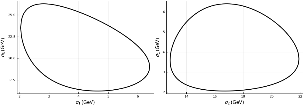
A natural way to visualize the three-body decay with two degrees of freedom is a correlation plot of the subchannel invariant masses squared. Kinematic limits can visualized using the border function. Plot in the σ₁σ₃ variables is obtained by

plot(
  plot(border31(tbs), xlab="σ₁ (GeV²)", ylab="σ₃ (GeV²)"),
  plot(border12(tbs), xlab="σ₂ (GeV²)", ylab="σ₁ (GeV²)"))

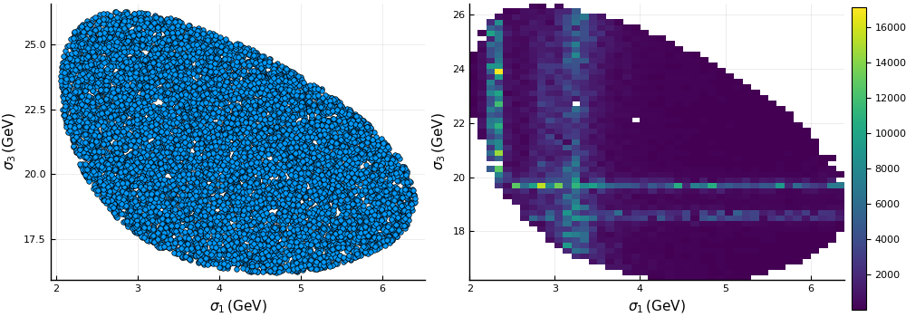
A phase-space sample is generated using the flatDalitzPlotSample function. By weighting the sample one gets the intensity distribution. The intensity function can also be plotted on the Dalitz plan using a grid.

using TypedTables # converint inteface of selecting columns
#
σsv = Table(flatDalitzPlotSample(tbs.ms; Nev = 10_000))
weights = I.(σsv) # dot is a broadcast
#
plot(layout=(900,350), layout=grid(1,2), xlab="σ₁ (GeV²)", ylab="σ₃ (GeV²)")
histogram2d!(sp=1, σsv.σ1, σsv.σ3, weights=weights, lab="weighted phase space"))
plot!(sp=2, I, tbs.ms; iσx=1, iσy=3, lab="on a grid")

mmikhasenko/ThreeBodyDecay.jl

ThreeBodyDecay

API for describing the decay

Plotting API