JumpProcesses.jl

Note, JumpProcesses.jl is a renaming of DiffEqJump.jl, providing the current version of the latter.

JumpProcesses.jl provides methods for simulating jump processes, known as stochastic simulation algorithms (SSAs), Doob's method, Gillespie methods, or Kinetic Monte Carlo methods across different fields of science. It also enables the incorporation of jump processes into hybrid jump-ODE and jump-SDE models, including jump diffusions.

JumpProcesses is a component package in the SciML ecosystem, and one of the core solver libraries included in DifferentialEquations.jl.

For information on using the package, see the stable documentation. Use the in-development documentation for the version of the documentation which contains unreleased features.

The documentation includes

a tutorial on simulating basic Poisson processes
a tutorial and details on using JumpProcesses to simulate jump processes via SSAs (i.e. Gillespie methods),
a tutorial on simulating jump-diffusion processes,
a reference on the types of jumps and available simulation methods,
a reference on jump time stepping methods,
a FAQ with information on changing parameters between simulations and using callbacks,
the JumpProcesses.jl API documentation.

Installation

There are two ways to install JumpProcesses.jl. First, users may install the meta DifferentialEquations.jl package, which installs and wraps OrdinaryDiffEq.jl for solving ODEs, StochasticDiffEq.jl for solving SDEs, and JumpProcesses.jl, along with a number of other useful packages for solving models involving ODEs, SDEs and/or jump process. This single install will provide the user with all of the facilities for developing and solving Jump problems.

To install the DifferentialEquations.jl package, refer to the following link for complete installation details.

If the user wishes to separately install the JumpProcesses.jl library, which is a lighter dependency than DifferentialEquations.jl, then the following code will install JumpProcesses.jl using the Julia package manager:

using Pkg
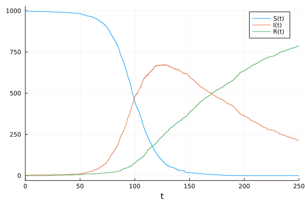
Pkg.add("JumpProcesses")

Examples

Stochastic Chemical Kinetics SIR Model

Here we consider the stochastic chemical kinetics jump process model for the basic SIR model, involving three species, $(S,I,R)$, that can undergo the reactions $S + I \to 2I$ and $I \to R$ (each represented as a jump process)

using JumpProcesses, Plots

# here we order S = 1, I = 2, and R = 3
# substrate stoichiometry:
substoich = [[1 => 1, 2 => 1],    # 1*S + 1*I
    [2 => 1]]            # 1*I
# net change by each jump type
netstoich = [[1 => -1, 2 => 1],   # S -> S-1, I -> I+1
    [2 => -1, 3 => 1]]   # I -> I-1, R -> R+1
# rate constants for each jump
p = (0.1 / 1000, 0.01)

# p[1] is rate for S+I --> 2I, p[2] for I --> R
pidxs = [1, 2]

maj = MassActionJump(substoich, netstoich; param_idxs = pidxs)

u₀ = [999, 1, 0]       #[S(0),I(0),R(0)]
tspan = (0.0, 250.0)
dprob = DiscreteProblem(u₀, tspan, p)

# use the Direct method to simulate
jprob = JumpProblem(dprob, Direct(), maj)

# solve as a pure jump process, i.e. using SSAStepper
sol = solve(jprob, SSAStepper())
plot(sol)

Instead of MassActionJump, we could have used the less efficient, but more flexible, ConstantRateJump type

rate1(u, p, t) = p[1] * u[1] * u[2]  # p[1]*S*I
function affect1!(integrator)
    integrator.u[1] -= 1         # S -> S - 1
    integrator.u[2] += 1         # I -> I + 1
end
jump = ConstantRateJump(rate1, affect1!)

rate2(u, p, t) = p[2] * u[2]      # p[2]*I
function affect2!(integrator)
    integrator.u[2] -= 1        # I -> I - 1
    integrator.u[3] += 1        # R -> R + 1
end
jump2 = ConstantRateJump(rate2, affect2!)
jprob = JumpProblem(dprob, Direct(), jump, jump2)
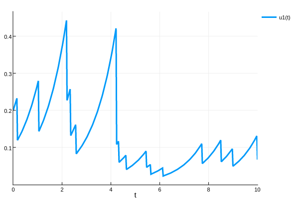
sol = solve(jprob, SSAStepper())

Jump-ODE Example

Let's solve an ODE for exponential growth, but coupled to a constant rate jump (Poisson) process that halves the solution each time it fires

using DifferentialEquations, Plots

# du/dt = u is the ODE part
function f(du, u, p, t)
    du[1] = u[1]
end
u₀ = [0.2]
tspan = (0.0, 10.0)
prob = ODEProblem(f, u₀, tspan)

# jump part

# fires with a constant intensity of 2
rate(u, p, t) = 2

# halve the solution when firing
affect!(integrator) = (integrator.u[1] = integrator.u[1] / 2)
jump = ConstantRateJump(rate, affect!)

# use the Direct method to handle simulating the jumps
jump_prob = JumpProblem(prob, Direct(), jump)

# now couple to the ODE, solving the ODE with the Tsit5 method
sol = solve(jump_prob, Tsit5())
plot(sol)

Contributing and Getting Help