Official Python implementation of the Delaunay Component Analysis (DCA) algorithm presented in the paper Delaunay Component Analysis for Evaluation of Data Representations. If you use this code in your work, please cite it as follows:
@inproceedings{
    poklukar2022delaunay,
    title={Delaunay Component Analysis for Evaluation of Data Representations},
    author={Petra Poklukar and Vladislav Polianskii and Anastasiia Varava and Florian T. Pokorny and Danica Kragic Jensfelt},
    booktitle={International Conference on Learning Representations},
    year={2022},
    url={https://openreview.net/forum?id=HTVch9AMPa}
}
Install the requirements with poetry:
poetry install
chmod +x dca/approximate_Delaunay_graph
Note: Delaunay graph building algorithm requires access to a GPU.
- Run a 2D example that saves the intermediate files:
poetry run python examples/first_example.py
- Check out the results saved
output/first_examplewhich will have the following structure:
experiments/first_example/
  /precomputed
    - clusterer.pkl               # HDBSCAN clusterer object
    - input_array.npy             # array of R and E points
    - input_array_comp_labels.npy # array of component labels corresponding to R and E points
    - unfiltered_edges.npy        # array of unfiltered approximated Delaunay edges
    - unfiltered_edges_len.npy    # array of unfiltered approximated Delaunay edge lengths
  /template_id1
    - output.json                 # dca scores
    /DCA
        - components_stats.pkl    # Local evaluation scores
        - network_stats.pkl       # Global evaluation scores
    /visualization
        - graph visualizations
    /logs
        - version0_elapsed_time.log      # empirical runtime
        - version0_input.json            # specific input parameters
        - version0_output_formatted.log  # all evaluation scores in a pretty format
        - version0_experiment_info.log   # console logs
        - # output files from qDCA
        - # any additional logs that should not be shared across experiment_ids in precomputed folder
Note: you can modify the experiment structure by definining what is shared across several experiments, e.g., what goes in the output/first_example/precomputed folder. For examples, see CL_ablation_study.py.
- In
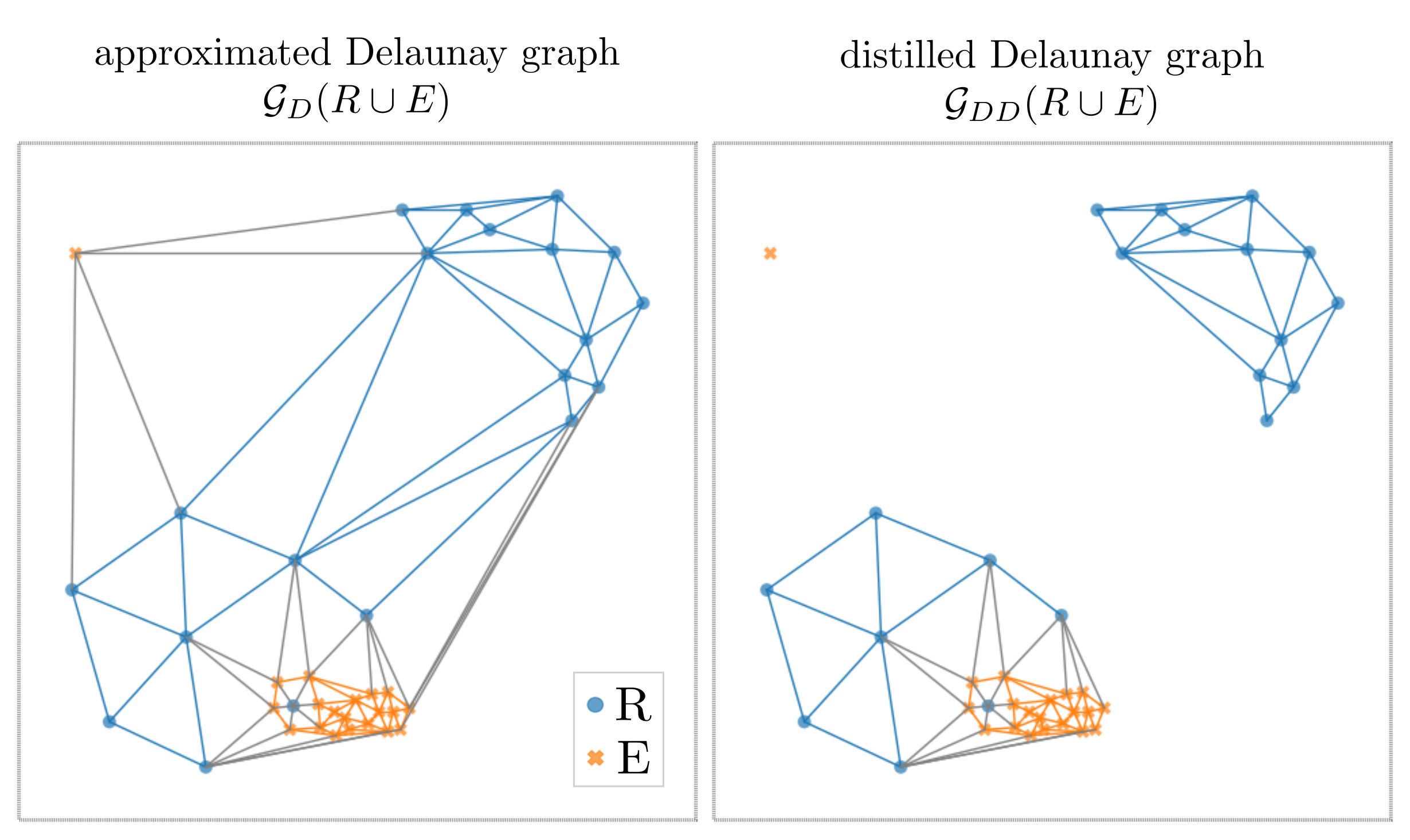
output/first_example/template_id1/visualizationfolder you should see an image of the approximated Delaunay graph and the distilled Delaunay graph like the ones below:
- In
output/first_example/template_id1/logs/version0_output_formatted.logyou should see the following output:
[mm/dd/yyyy hh:mm:ss] :: num_R: 20                            # total number of R points
[mm/dd/yyyy hh:mm:ss] :: num_E: 20                            # total number of E points
[mm/dd/yyyy hh:mm:ss] :: precision: 0.95
[mm/dd/yyyy hh:mm:ss] :: recall: 0.4
[mm/dd/yyyy hh:mm:ss] :: network_consistency: 1.0
[mm/dd/yyyy hh:mm:ss] :: network_quality: 0.2
[mm/dd/yyyy hh:mm:ss] :: first_trivial_component_idx: 2       # idx of the first outlier
[mm/dd/yyyy hh:mm:ss] :: num_R_points_in_fundcomp: 8          # number of vertices in F^R
[mm/dd/yyyy hh:mm:ss] :: num_E_points_in_fundcomp: 19         # number of vertices in F^E
[mm/dd/yyyy hh:mm:ss] :: num_RE_edges: 19                     # number of heterogeneous edges in G_DD
[mm/dd/yyyy hh:mm:ss] :: num_total_edges: 95                  # number of all edges in G_DD
[mm/dd/yyyy hh:mm:ss] :: num_R_outliers: 0
[mm/dd/yyyy hh:mm:ss] :: num_E_outliers: 1
[mm/dd/yyyy hh:mm:ss] :: num_fundcomp: 1                      # number of fundamental components |F|
[mm/dd/yyyy hh:mm:ss] :: num_comp: 3                          # number of all connected components
[mm/dd/yyyy hh:mm:ss] :: num_outliercomp: 1                   # number of trivial components
# Local scores for each component G_i: consistency and quality (Def 3.2) as well as number of R and E points contained in it
[mm/dd/yyyy hh:mm:ss] :: c(G0): 0.59, q(G0): 0.27, |G0^R|_v: 8   , |G0^E|_v: 19  , |G0|_v: 27
[mm/dd/yyyy hh:mm:ss] :: c(G1): 0.00, q(G1): 0.00, |G1^R|_v: 12  , |G1^E|_v: 0   , |G1|_v: 12
[mm/dd/yyyy hh:mm:ss] :: c(G2): 0.00, q(G2): 0.00, |G2^R|_v: 0   , |G2^E|_v: 1   , |G2|_v: 1
- If you are only interested in the output DCA scores, the
cleanupfunction will remove all of the intermediate files for you. Test it on this 2D example by running
poetry run python examples/first_example.py --cleanup 1
Note: to run q-DCA it is required to keep the intermediate files. This is because the distilled Delaunay graph is needed to calculate edges to the query points.
Minimum example requires you to define the input parameters as in the code below. See dca/schemes.py for the optional arguments of the input configs.
# Generate input parameters
data_config = REData(R=R, E=E)
experiment_config = ExperimentDirs(
    experiment_dir=experiment_path,
    experiment_id=experiment_id,
)
graph_config = DelaunayGraphParams()
hdbscan_config = HDBSCANParams()
geomCA_config = GeomCAParams()

# Initialize loggers
exp_loggers = DCALoggers(experiment_config.logs_dir)

# Run DCA
dca = DCA(
    experiment_config,
    graph_config,
    hdbscan_config,
    geomCA_config,
    loggers=exp_loggers,
)
dca_scores = dca.fit(data_config)
dca.cleanup()  # Optional cleanup
We used and adjusted datasets used in our eariler work GeomCA. Therefore, we only provide the representations used in the contrastive learning experiment and q-DCA stylegan experiment, which you can download on this link and save them in representations/contrastive_learning and representations/stylegan folders, respectively. For VGG16, we provide the code (see VGG16_utils.py) we used on the splits constructed in GeomCA. For StyleGAN mode truncation experiment, we refer the user either to the splits we provided in GeomCA or to the code provided by Kynkäänniemi et. al.
Reproduce Varying component density experiment:
poetry run python experiments/contrastive_learning/CL_varying_component_density.py --n-iterations 10 --perc-to-discard 0.5 --cleanup 1
Reproduce Cluster assignment experiment, for example, using query set Q2 and considering flexible assignment procedure:
poetry run python experiments/contrastive_learning/CL_qDCA.py Df query_Df_holdout_c7_to_c11 --run-dca 1 --run-qdca 1 --several-assignments 1 --cleanup 1
Reproduce Mode truncation experiment in Appendix B.1:
poetry run python experiments/contrastive_learning/CL_mode_truncation.py --cleanup 1
Reproduce Ablation study experiments in Appendix B.1:
poetry run python experiments/contrastive_learning/CL_ablation_study.py cl-ablation-delaunay-edge-approximation --cleanup 1
poetry run python experiments/contrastive_learning/CL_ablation_study.py cl-ablation-delaunay-edge-filtering --cleanup 1
poetry run python experiments/contrastive_learning/CL_ablation_study.py cl-ablation-hdbscan --cleanup 1
Reproduce Mode truncation experiment, for example, on truncation 0.5 and 5000 representations provided by Poklukar et. al in GeomCA:
poetry run python experiments/stylegan/StyleGAN_mode_truncation.py 0.5 --num-samples "5000" --cleanup 1
Reproduce Quality of individual generated images experiment using qDCA, for example, on truncation 0.5 --cleanup 1
poetry run python experiments/stylegan/StyleGAN_qDCA.py --run-dca 1 --run-qdca 1 --cleanup 1
Reproduce Class separability experiment, for example, on version 1 containing classes of dogs and kitchen utils
poetry run python experiments/vgg16/VGG16_class_separability.py --version-id 1 --cleanup 1
Reproduce Amending labelling inconsistencies experiment using qDCA, for example, on version 1 containing classes of dogs and kitchen utils
poetry run python experiments/vgg16/VGG16_qDCA.py --version-id 1 --run-dca 1 --run-qdca 1 --cleanup 1
