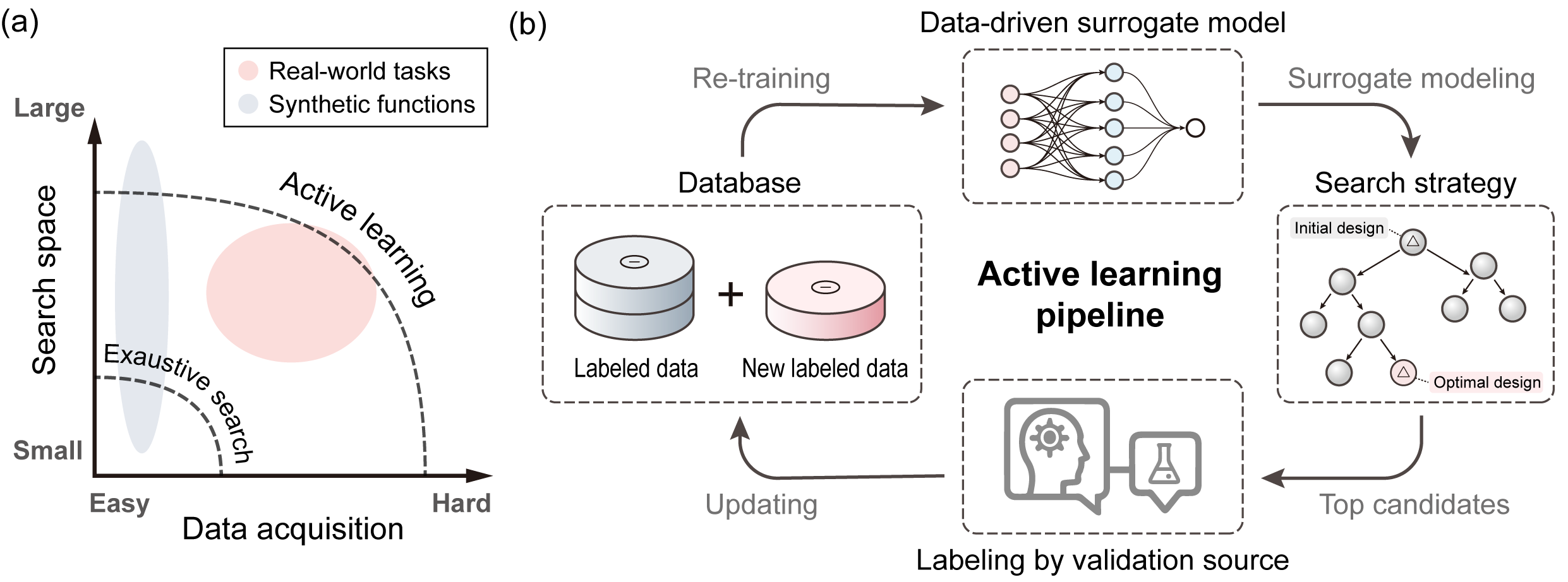
BALSA is a comprehensive benchmark suite for evaluating active learning and optimisation algorithms in real-world scientific design tasks, with a focus on materials science and biology. The suite provides standardised implementations, metrics, and evaluation protocols to enable systematic comparison of different approaches.
- Real-world Scientific Tasks: Includes challenging tasks from electron ptychography and protein design
- Synthetic Benchmark Functions: Standard test functions with known properties and varying difficulty
- Standardised Evaluation: Consistent protocols for fair algorithm comparison
- Active Learning Framework: Easy integration of new tasks and algorithms
- Comprehensive Baselines: Implementation of 10+ state-of-the-art optimisation methods
Comparison of reconstructed phases (object transmission functions) obtained using different derivative-free optimisation methods on a MoS₂ dataset. Results demonstrate the relative performance of various approaches in this high-dimensional (14D) optimisation task.
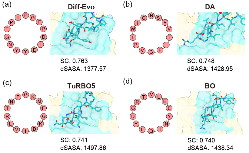
Performance comparison of different optimisation strategies for designing cyclic peptide binders, showing the peptide sequences and corresponding protein interaction maps for target protein 4kel.
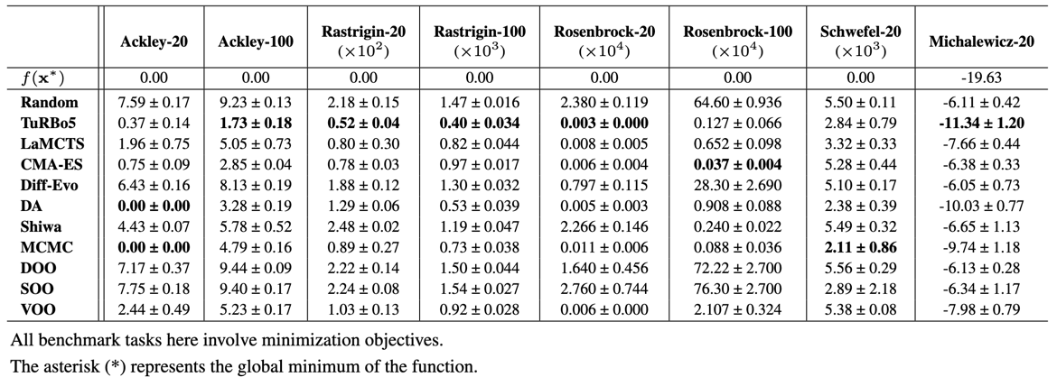
Quantitative comparison across standard test functions. Results show mean ± standard deviation over 5 independent trials.
- Python ≥ 3.12
- CUDA-enabled GPU (recommended)
- TensorFlow and Keras with GPU support
For most users, the basic installation is sufficient:
pip install -e "git+https://github.com/poyentung/balsa.git"If you plan to contribute or need additional development tools:
# Option 1: Direct installation with dev dependencies
pip install -e "git+https://github.com/poyentung/balsa.git#egg=balsa[dev]"

# Option 2: Clone and install locally
git clone https://github.com/poyentung/balsa.git
cd balsa
pip install -e ".[dev]"
Note: If you want to test cyclic peptide design, make sure you have ColabDesign and PyRosetta installed.
Refer to https://github.com/sokrypton/ColabDesign/tree/main/af for ColabDesign.
Refer to https://www.pyrosetta.org/downloads for PyRosetta.
Run the test suite to ensure everything is working correctly:
# Basic tests (recommended for most users)
python -m pytest -m "not slow and not dev"

# Extended tests (for developers)
python -m pytest -m "not slow"

# Full test suite (for developers)
python -m pytest
Note: The basic test suite is sufficient for most users. Extended and full tests are primarily for development purposes and may take longer to complete.
This example demonstrates how to optimise parameters for electron ptychography reconstruction using the TuRBO algorithm. The task involves:
- Optimising 14 reconstruction parameters for the MoS₂ dataset
- Using a sequential acquisition strategy with 20 iterations (1 new sample per iteration)
- Starting with 30 initial random samples
python scripts/run_ptycho.py search_method=turbo \
                             obj_func_name=ptycho \
                             dims=14 \
                             num_acquisitions=50 \
                             num_samples_per_acquisition=1 \
                             num_init_samples=30
Note: For TuRBO and LaMCTS algorithms, the total number of samples (num_acquisitions × num_samples_per_acquisition) represents the complete budget including initial samples. The total number of new samples should be num_acquisitions × num_samples_per_acquisition - num_init_samples (30 - 20).
This example shows how to benchmark multiple optimisation algorithms on the Ackley function, a standard test problem with a pre-defined surrogate model:
- Compares MCMC, CMA-ES, and Dual Annealing approaches
- Optimises in 10 dimensions
- Uses 50 initial random samples
- Performs 10 acquisition iterations
- Collects 20 samples per iteration (200 total evaluations)
python scripts/run.py -m search_method=mcmc,cmaes,da \
                         obj_func_name=ackley \
                         dims=10 \
                         num_acquisitions=100 \
                         num_samples_per_acquisition=20 \
                         num_init_samples=50
Results will be saved in the results directory, including performance metrics and optimisation trajectories for each algorithm.
We provide detailed tutorials to help you get started with BALSA:
- Adding Custom Functions - Learn how to create and integrate your own optimisation functions
- Custom Function Configuration - Detailed guide on configuring and running custom functions
- Jupyter notebook - Jupyter notebook version of the custom function tutorial
For a quick start, here's a basic example of creating a custom function. For detailed instructions, see our Custom Functions Tutorial.
@dataclass
class CustomObjectiveFunction(ObjectiveFunction):
    """Custom objective function for optimisation."""
    name: str = "custom_objective"
    turn: float = 0.1  # Controls input discretisation granularity

    def __post_init__(self):
        super().__post_init__()
        # Define problem bounds
        self.lb = -5 * np.ones(self.dims)  # Lower bounds
        self.ub = 5 * np.ones(self.dims)   # Upper bounds

    @override
    def _scaled(self, y: float) -> float:
        """Scale objective value for surrogate fitting."""
        return 1 / (y + 0.01)  # For minimisation problems
        # return -1 * y  # For maximisation problems

    @override
    def __call__(self, x: NDArray, saver: bool = True, return_scaled: bool = False) -> float:
        """Compute objective value for given input."""
        x = np.array(x / self.turn).round(0) * self.turn  # Discretise input values
        self.counter += 1

        y = float(your_objective_function(x))  # Your function here

        self.tracker.track(y, x, saver)
return y if not return_scaled else self._scaled(y)- Set appropriate bounds (
lb,ub) for your problem - Choose scaling based on whether you're minimising or maximising
- Use
self.trackerto log evaluations - The
turnparameter controls input discretisation:turn = 0.1: Rounds inputs to nearest 0.1 (e.g., 1.23 → 1.2)turn = 1.0: Rounds to integers- Smaller values allow finer granularity but increase search space
- Electron Ptychography: 14-dimensional parameter optimisation for microscopy reconstruction
- Cyclic Peptide Design: Protein engineering for targeted binding
- Ackley
- Rastrigin
- Rosenbrock
- Schwefel
- Michalewicz
- Griewank
We welcome contributions! Please submit a PR to:
- Add new scientific tasks
- Implement additional algorithms
- Improve documentation
- Fix bugs
This project is licensed under the MIT License - see the LICENSE file for details.


