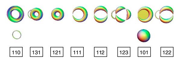
In the early of 20th century Algebraic topology provided, thanks to Poincaré, a general framework to classify shapes. Indeed the Euler characteristic equal to the alternating sum of the Betti numbers is a topological invariant. Roughly these numbers count the number of distinct objects in the domain, the number of holes and the number of voids they contain etc...
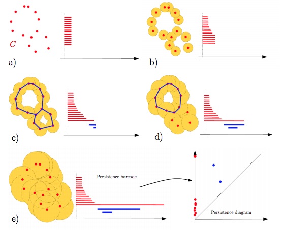
Topological Data Analysis (TDA) is the field which apply these theorical tools in order to proceed data analysis. But these latter characteristics cannot be used straight forward because of the uncertainty of the datas and because of the sensitivity of Betti numbers to minor outliers in the data set. Therefore to tackle this issue the main tool TDA is using is persistent homology, in which the invariants are in the form of persistence diagrams also called barcodes. Topological invariants will then quantify the stability of geometric features with respect to degradation such as noise or artefacts
Credits @ Frédéric Chazal, Bertrand Michel
We used TDA framework to perform unsupervised image segmentation. The set of images provided by the skimage library from python and the python library Gudhi @INRIA to produce simplicial complexes and persistence diagrams.
The main procedure was as followed :
- Apply a small gaussian blur to the image to remove isolated pixels (outliers)
- Take a random sample of points from the image called superpixels. We obtain a 3D cloud point if image is gray a 5D cloud point if the image is in color.
- Compute the Nested Rips-Vietoris complexes from those points
- Computed nested RV complexes for radius ε from 0 to infinity
- Set a value for edges : the distance between the two vertices. Value of vertices is set to 0.
- Set a value for each simplex by taking the max value of all its edges (Method called age filter)
- Compute the persistent pairs for homology groups for dimensions 0 and 1 and for 1 and 2.
- For dimensions 0 and 1 these are pairs (c,e) where e is an edge that vanish a connected component c (represented by its first vertex).
- For dimensions 1 and 2 these are pairs (c,e) where e is an edge that vanish a 1-loop c (represented by its first vertex).
- We compute the graph from the set of all edges of persistent pairs of dimensions 0-1. In fact it is equivalent as computing the covering tree of the 1-skeleton of our RV-complex, that is to say the covering tree over our cloud data point with minimum value.
- In order to compute most persistent connected components and loops we then apply different procedures:
- For connected components we compute the graph from the set of all edges of persistent pairs of dimensions 0-1. In fact it is equivalent as computing the covering tree of the 1-skeleton of our RV-complex, that is to say the covering tree over our cloud data point with minimum value.Then removing n − 1 edges from this tree in decreasing order of value gives us the n most persistent connected components.
- For cycles we add edges which give birth to the most persistent cycles through the filtration. Then we find loops with a traversal algorithm
- The most persistent connected components and the most persistent cycles give each a segmentation of our images.
Please note that in practice to compute most relevant and persistent 0 homology groups we followed two more steps we don't develop:
- to compute most relevant connected components we actually use a tree where each split represents a persistence pair and we use gini criterion to select most relevant ones
- we use a sampling method based on empirical distribution of superpixel labels to infer labels on every pixels from image
Note: since computation was heavy for our computer we had to use only 5000 to 10000 superpixels that is 2% to 4% of all pixels. It is interesting to see that we still managed to get decent results while TDA researchers actually use all pixels into their computation.
Here is one example of image segmentation produced using the naive procedure. It produced 250 most persistent 0th homology groups but they are irrelevant. These are isolated pixels.
Here we removed isolated pixels. We then applied our sampling method to recover labels for these as well. We have a more parsimonious segmentation with 21 segments but they are not homogeneous as a large part of image remains as one segment.
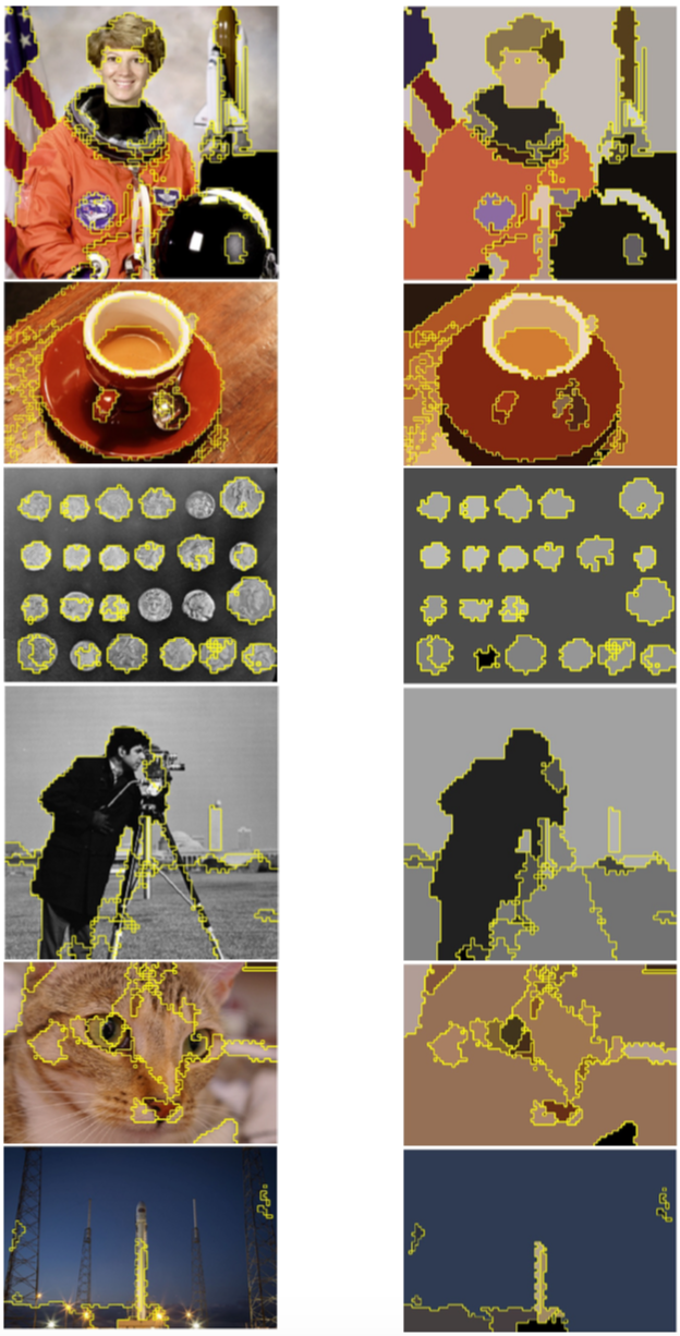
Here are our final results for 0th homology groups where we applied full procedure. We used the same parameters for all images. Results are parsimonious as we get between 10 and 30 segments and they are more homogenous.
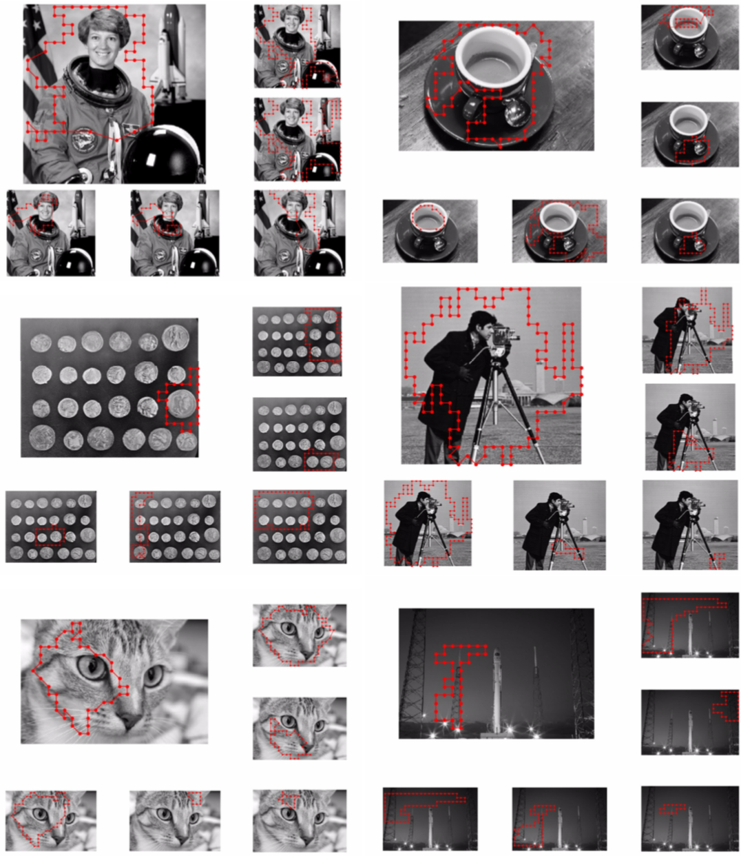
Here are our final results for 1th homology groups where we applied full procedure. Actually we noticed that most often only the most persistent cycle may be relevant to the image. Although the main drawback with 1th homology groups is that a relevant cycle in 3D or 5D RV complex may become irrelevant when projected into 2D.
To conclude we found that topological persistence of 0 dimension elements is an effective and robust (no need of parameter tuning) method for image segmentation but more generally for unsupervised data processing. Also it is interesting to see that this method is close to Felzenswalb's algorithm. It provides a theorical framework which explains why this algorithm is so powerful. In the contrary we found that topological persistence of 1 dimension elements is not useful in the case of images due to projection issue.


