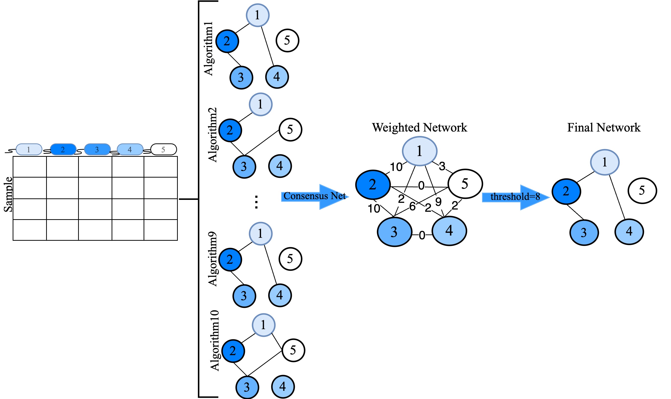
The package employs a range of established algorithms, including Pearson and Spearman correlation, Biweight midcorrelation, Sparse Correlations for Compositional data (SparCC), Sparse InversE Covariance estimation for Ecological Association and Statistical Inference (SpiecEasi), Semi-Parametric Rank-based Correlation and Partial Correlation Estimation (SPRING), Generalized Co-Occurrence Differential Abundance analysis (gCoda), Correlation Inference for Compositional Data through Lasso (CCLasso), and a novel algorithm based on conditional mutual information (c_MI). These algorithms construct individual microbial association networks, which CMiNet then combines into a single, weighted consensus network. By leveraging the strengths of each method, CMiNet provides a comprehensive and reliable representation of microbial interactions.
Algorithms Applied in CMiNet:
- Pearson coefficient (cor() from stats package)
- Spearman coefficient (cor() from stats package)
- Biweight Midcorrelation (bicor() from WGCNA package)
- SparCC (R code on GitHub)
- CCLasso (R code on GitHub)
- SpiecEasi (SpiecEasi package)
- SPRING (SPRING package)
- CMIMN (CMIMN package)
- gCoda (R code on GitHub)
install.packages("devtools")
devtools::install_github("solislemuslab/CMiNet")
If there are any errors during installation, please install the missing dependencies manually. In particular the automatic installation of SPRING and SpiecEasi (only available on GitHub) does sometimes not work. These packages can be installed as follows (the order is important because SPRING depends on SpiecEasi):
devtools::install_github("zdk123/SpiecEasi@v1.1.1")
devtools::install_github("GraceYoon/SPRING")
if (!requireNamespace("BiocManager", quietly = TRUE))
    install.packages("BiocManager")
BiocManager::install(c("AnnotationDbi", "GO.db", "preprocessCore", "impute"))
library(AnnotationDbi)
library(GO.db)
library(preprocessCore)
library(impute)
library(SpiecEasi)
library(SPRING)To ensure all output files and figures are saved automatically and organized properly, we recommend opening a new R project. This setup will help organize the generated files, as CMiNet will automatically save figures and outputs in the current working directory. If you prefer to specify a different path for saving the output (e.g., the Binary_network files), you can manually set the path in your code.
-
CMiNet: This function constructs a consensus network from microbiome data using multiple methods.
-
process_and_visualize_network: This function processes a weighted microbiome network and visualizes it across different thresholds. Each threshold represents a minimum edge weight required for inclusion in the network plot.
-
plot_hamming_distances: Calculates the Hamming distance, common edges, and the number of edges for each pair of resulting network matrices.
-
plot_network: This function generates a network plot from a final network produced by CMiNet.
We use the American Gut data from SpiecEasi package to run CMiNet algorithm to construct consensus microbiome network. First, load CMiNet and the American Gut Project data (included with the SpiecEasi package), which is automatically loaded alongside CMiNet).
library(SpiecEasi)
library(SPRING)
library(CMiNet)
data = amgut1.filt
taxa_name <- matrix(0, nrow = dim(data)[2], ncol = 2)
taxa_name[, 1] <- colnames(data)
taxa_name[, 2] <- 1:dim(data)[2]
colnames(taxa_name) <- c("original", "figures_name")We designed the package to allow users to adjust the default parameters of each algorithm according to their preferences and specific research needs.
- sparcc_params = list(imax = 20, kmax = 10, alpha = 0.1, Vmin = 1e-4)
- spiecEasi_mb_params= list(method = 'mb', lambda.min.ratio = 1e-2, nlambda = 15, pulsar.params = list(rep.num = 20, ncores = 4))
- spiecEasi_glasso_params =params = list(method = 'glasso', lambda.min.ratio = 1e-2, nlambda = 15, pulsar.params = list(rep.num = 50))
- spring_params = list(Rmethod = "original", quantitative = TRUE, ncores = 5, lambdaseq = "data-specific", nlambda = 15, rep.num = 20)
- gcoda_params = list(counts = FALSE, pseudo = 0.5, lambda.min.ratio = 1e-4, nlambda = 15, ebic.gamma = 0.5)
- c_MI_params = list(quantitative = TRUE, q1 = 0.7, q2 = 0.95)
- cclasso_params = list(counts = FALSE, pseudo = 0.5, k_cv = 3, lam_int = c(1e-4, 1), k_max = 20, n_boot = 20)
- Description: The CMiNet function constructs a consensus network from microbiome data by integrating multiple network construction algorithms. This approach combines individual microbial association networks into a single weighted network, enhancing reliability by leveraging the strengths of each method.
- Parameters:
- data: The input microbiome abundance matrix, where rows represent samples and columns represent taxa.
- quantitative (default = TRUE): Set to TRUE if the data contains quantitative abundance counts; set to FALSE otherwise.
- TT: The threshold value used for threshold-dependent algorithms (pearson, spearman, bicor, SparCC, and CCLasso), set to the 0.95 quantile by default to promote sparsity in the consensus network.
- Algorithm-Specific Parameters:
- pearson, spearman, bicor: Boolean flags to enable these correlation-based methods. When set to TRUE, the algorithm runs on the data; when set to FALSE, it is excluded from the analysis.
- SparCC, SpiecEasi_mb, SpiecEasi_glasso, SPRING, gCoda, c_MI, CCLasso: Lists of parameters for each algorithm, allowing customization of settings such as number of cores (ncores), threshold values (lambda.min.ratio), and other algorithm-specific configurations.
- Setting the enabled parameter to TRUE for an algorithm will include it in the consensus network construction, while setting it to FALSE will skip the algorithm, allowing users to select a subset of methods for analysis.
- Returns: A list containing:
- weighted_network: A weighted network matrix representing the consensus network.
- edge_list: A matrix with three columns—first and second columns indicate node IDs, and the third column shows the edge weight values.
- errors: Any errors from algorithms that could not run on the data, providing feedback for troubleshooting.
sparcc_params = list(imax = 20, kmax = 10, alpha = 0.1, Vmin = 1e-4)
spiecEasi_mb_params= list(method = 'mb', lambda.min.ratio = 1e-2, nlambda = 15, pulsar.params = list(rep.num = 20, ncores = 4))
spiecEasi_glasso_params =params = list(method = 'glasso', lambda.min.ratio = 1e-2, nlambda = 15, pulsar.params = list(rep.num = 50))
spring_params = list(Rmethod = "original", quantitative = TRUE, ncores = 5, lambdaseq = "data-specific", nlambda = 15, rep.num = 20)
gcoda_params = list(counts = FALSE, pseudo = 0.5, lambda.min.ratio = 1e-4, nlambda = 15, ebic.gamma = 0.5)
c_MI_params = list(quantitative = TRUE, q1 = 0.7, q2 = 0.95)
cclasso_params = list(counts = FALSE, pseudo = 0.5, k_cv = 3, lam_int = c(1e-4, 1), k_max = 20, n_boot = 20)
result <- CMiNet(
data,
quantitative = TRUE,
TT = 0.95,
pearson = list(enabled = TRUE),
spearman = list(enabled = TRUE),
bicor = list(enabled = TRUE),
sparcc = list(enabled = TRUE,params=sparcc_params),
spiecEasi_mb = list(enabled = TRUE,params = spiecEasi_mb_params),
spiecEasi_glasso = list(enabled = TRUE,params = spiecEasi_glasso_params),
spring = list(enabled = TRUE,params = spring_params),
gcoda = list(enabled =TRUE, params =gcoda_params),
c_MI = list(enabled =TRUE,params=c_MI_params),
cclasso = list(enabled = TRUE,params=cclasso_params)
)-
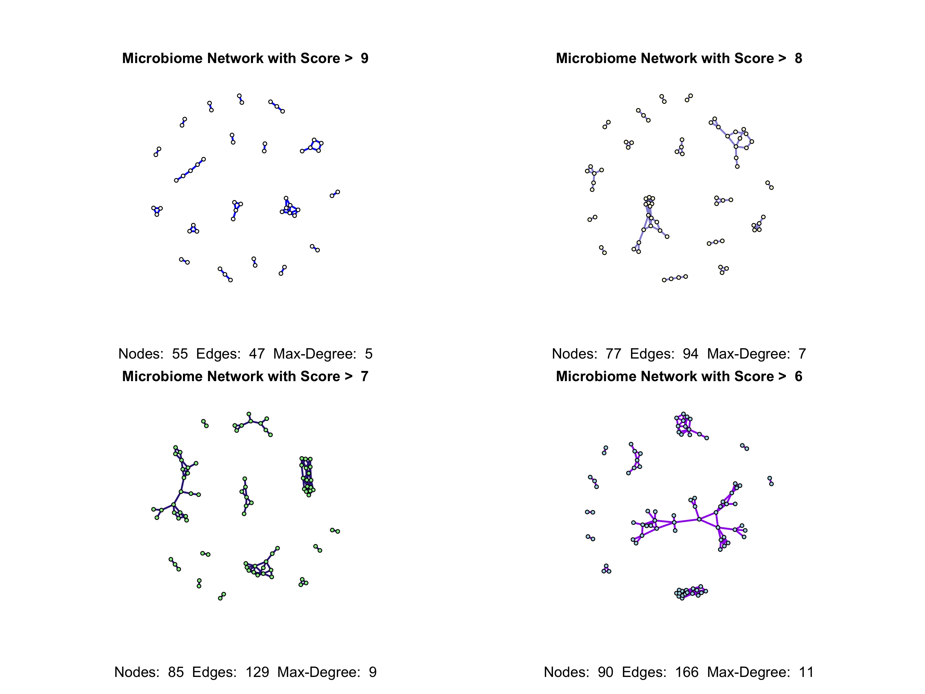
Description: The process_and_visualize_network function processes a weighted microbiome network and visualizes it across specified thresholds. Each threshold filters edges based on minimum weight, helping to analyze network structure at varying levels of connectivity.
-
Parameters:
- weighted_network: The input weighted network matrix generated by the CMiNet function.
- taxa_names: Vector of taxa names for labeling nodes in the network.
- thresholds: A vector of threshold values defining minimum edge weights for inclusion in the network plot.
- show_labels: Boolean vector indicating whether to display taxa names for each threshold (e.g., TRUE or FALSE).
- node_colors: Vector of colors for nodes in each threshold-based plot.
- edge_colors: Vector of colors for edges in each threshold-based plot.
-
Returns: A set of network plots for each threshold, visualizing taxa relationships based on edge weights. Each plot includes details on the number of nodes and edges in the network, and also the maximum degree value .
weighted_network = result$weighted_network
taxa_names <- taxa_name[, 2]
rownames(weighted_network) = colnames(weighted_network)=taxa_names
thresholds <- c(max(weighted_network)-1,max(weighted_network)-2,max(weighted_network)-3,max(weighted_network)-4)  # Thresholds for visualization
show_labels <- c(FALSE, FALSE, FALSE, FALSE)  # Show taxa names (TRUE/FALSE) for each threshold
node_colors <- c("white", "lightyellow",  "lightgreen","lightblue")  # Node colors for each threshold
edge_colors <- c("blue", "#9491D9", "#332288", "purple")  # Edge colors for each threshold
process_and_visualize_network(weighted_network, taxa_names, thresholds, show_labels, node_colors, edge_colors)-
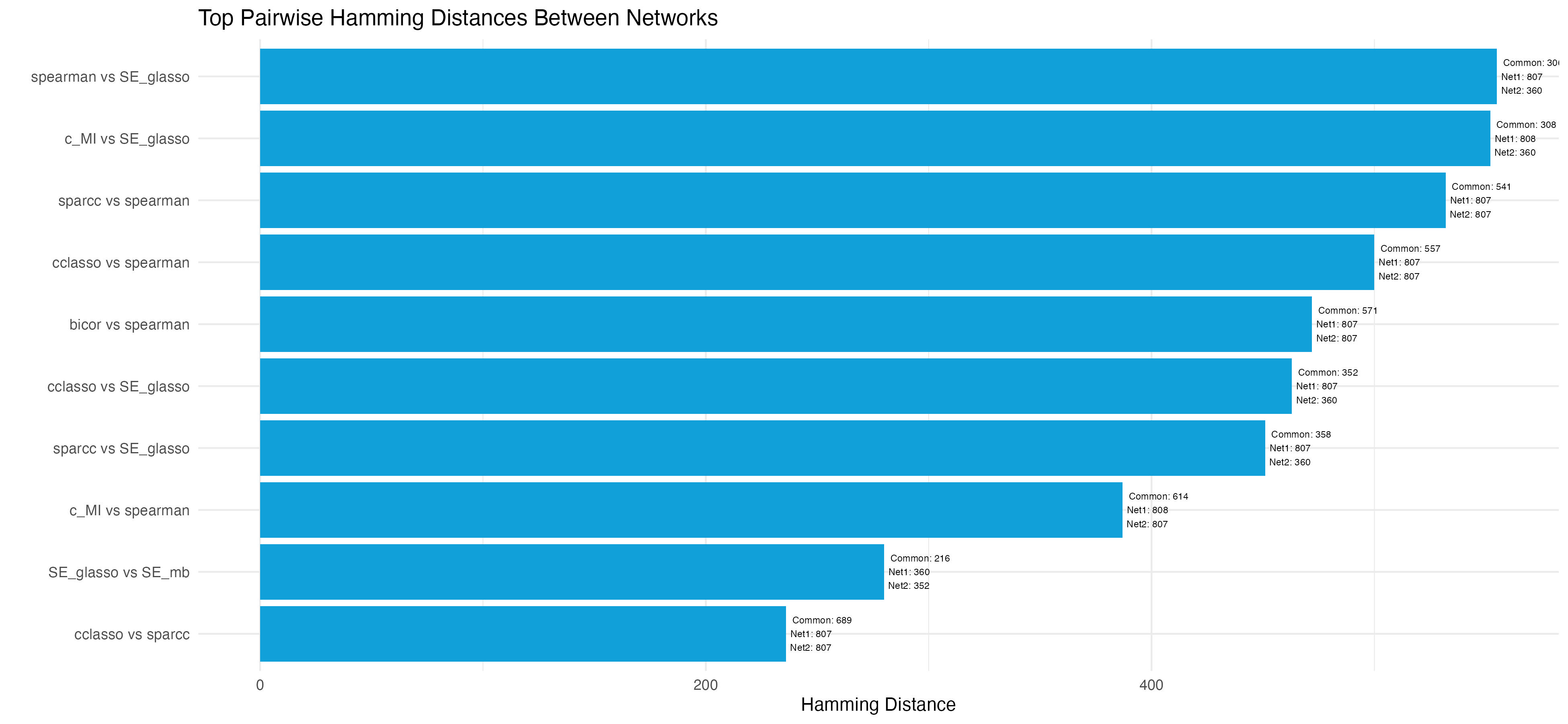
Description: The plot_hamming_distances function calculates the Hamming distance, number of common edges, and total edges for each pair of network matrices. It generates a plot to visualize these distances, providing insights into structural differences between networks generated by different algorithms or parameters.
-
Parameters:
- network_type (e.g., "Binary_Network"): The directory or folder where all the binary network matrices are saved.
- top_n_pairs: An integer specifying the top number of network pairs to display based on the smallest Hamming distances.
- output_filename: The filename for saving the Hamming distances plot as an image file.
-
Returns: A plot visualizing the Hamming distances between selected network pairs. The plot is optionally saved as an image file to the specified output_filename.
plot_hamming_distances("Binary_Network", top_n_pairs = 10, output_filename = "hamming_distances_plot.jpeg")-
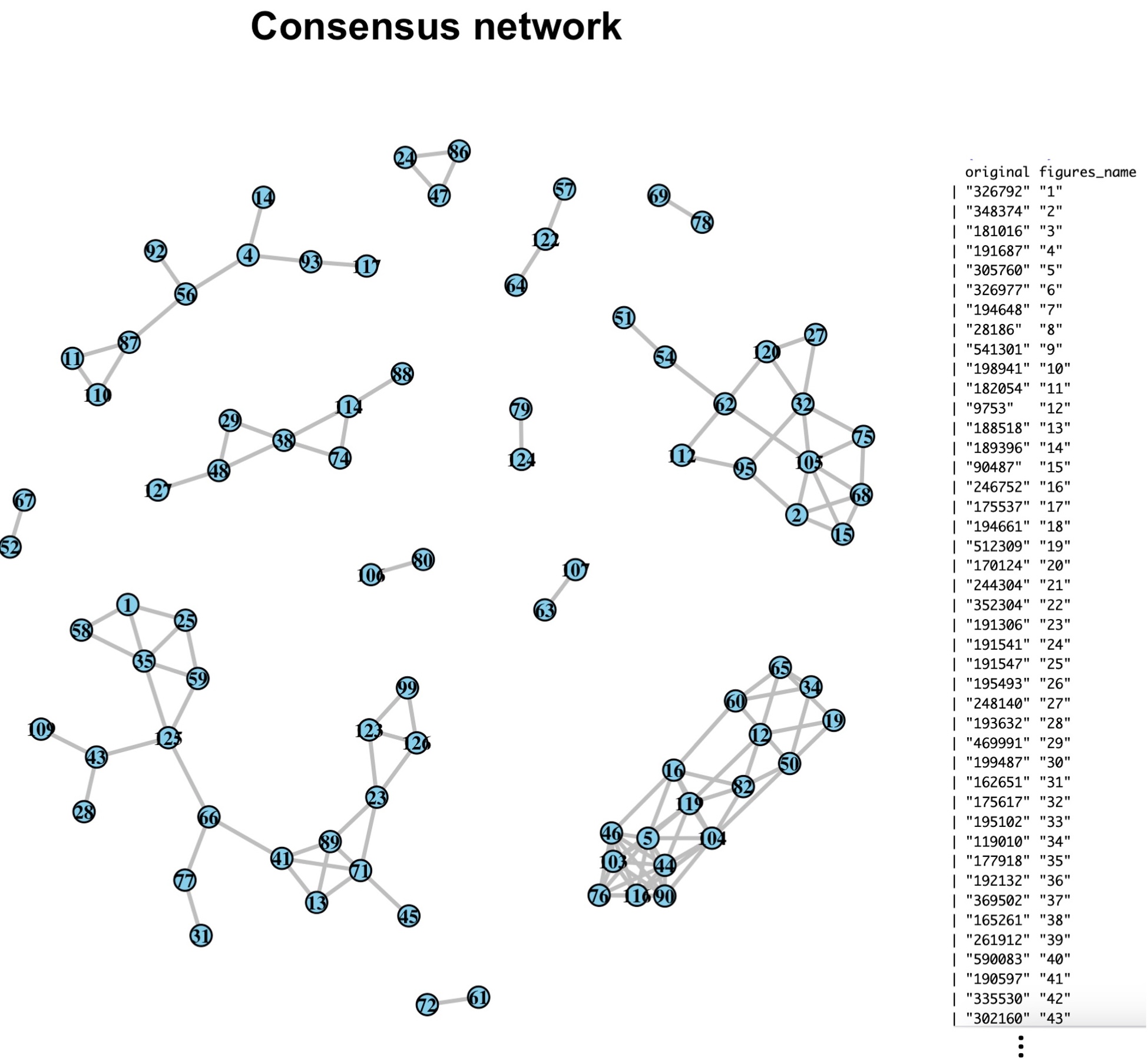
Description: The plot_network function generates a visual representation of the final consensus network by applying a score threshold. This threshold filters the network to display only the most significant edges, allowing users to examine the core structure of the microbiome network based on selected nodes and edges.
-
Parameters:
- network_final: A binarized network matrix derived from the weighted consensus network. The matrix is filtered based on a numeric Score threshold, where only edges with weights above this threshold are included.
- node_color: Specifies the color for nodes in the plot.
- edge_color: Specifies the color for edges in the plot.
- label_color: Specifies the color for node labels in the plot.
-
Returns: A figure displaying the final microbiome network, filtered by the score threshold. Nodes, edges, and labels are color-coded according to the specified parameters, providing a clear view of significant interactions within the network.
WN = result$weighted_network
taxa_names <- taxa_name[, 2]
rownames(WN) = colnames(WN)=taxa_names
score = max(WN)-3
network_final <- ifelse(WN > score, 1, 0)
network_final[lower.tri(network_final)] <- 0  # Only upper triangle will have non-zero values
sum(network_final)
plot_network(network_final, node_color = "skyblue", edge_color = "grey", label_color = "black")
You can print the original and formatted taxa names using the following command:
print(taxaname)If you encounter a bug, experience a failed function, or have a feature request, please open an issue in the GitHub issue tracker.
CMIMN is licensed under the GNU General Public License v3.0 (GPL-3). © Solis-Lemus Lab (2024).
If you use CMiNet in your work, we kindly ask that you cite the following paper:
@article{aghdam2024,
  year = {2024},
  publisher = {In process},
  author = {Rosa Aghdam, Shan Shan, Richard Lankau and Claudia Solis-Lemus},
  title = {Leveraging Machine Learning and Enhanced Network-based methods in Potato Disease Interactions}
}
@article{aghdam2024_2,
  year = {2024},
  publisher = {In process},
  author = {Rosa Aghdam and Claudia Solis-Lemus},
  title = {CMiNet: R package for learning the Consensus Microbiome Network}
} 


