loss-landscape-anim lets you create animated optimization path in a 2D slice of the loss landscape of your neural networks. It is based on PyTorch Lightning, please follow its suggested style if you want to add your own model.
Check out my article Visualizing Optimization Trajectory of Neural Nets for more examples and some intuitive explanations.
From PyPI:
pip install loss-landscape-animFrom source, you need Poetry. Once you cloned this repo, run the command below to install the dependencies.
poetry installWith the provided spirals dataset and the default multilayer perceptron MLP model, you can directly call loss_landscape_anim to get a sample animated GIF like this:
# Use default MLP model and sample spirals dataset
loss_landscape_anim(n_epochs=300)
Note: if you are using it in a notebook, don't forget to include the following at the top:
%matplotlib notebookHere's another example – the LeNet5 convolutional network on the MNIST dataset. There are many levers you can tune: learning rate, batch size, epochs, frames per second of the GIF output, a seed for reproducible results, whether to load from a trained model, etc. Check out the function signature for more details.
bs = 16
lr = 1e-3
datamodule = MNISTDataModule(batch_size=bs, n_examples=3000)
model = LeNet(learning_rate=lr)

optim_path, loss_steps, accu_steps = loss_landscape_anim(
    n_epochs=10,
    model=model,
    datamodule=datamodule,
    optimizer="adam",
    giffps=15,
    seed=SEED,
    load_model=False,
    output_to_file=True,
    return_data=True,  # Optional return values if you need them
    gpus=1  # Enable GPU training if available
)
GPU training is supported. Just pass gpus into loss_landscape_anim if they are available.
The output of LeNet5 on the MNIST dataset looks like this:
To create a 2D visualization, the first thing to do is to pick the 2 directions that define the plane. In the paper Visualizing the Loss Landscape of Neural Nets, the authors argued why 2 random directions don't work and why PCA is much better. In summary,
-
2 random vectors in high dimensional space have a high probability of being orthogonal, and they can hardly capture any variation for the optimization path. The path’s projection onto the plane spanned by the 2 vectors will just look like random walk.
-
If we pick one direction to be the vector pointing from the initial parameters to the final trained parameters, and another direction at random, the visualization will look like a straight line because the second direction doesn’t capture much variance compared to the first.
-
If we use principal component analysis (PCA) on the optimization path and get the top 2 components, we can visualize the loss over the 2 orthogonal directions with the most variance.
For showing the most motion in 2D, PCA is preferred. If you need a quick recap on PCA, here's a minimal example you can go over under 3 minutes.
Although PCA is a good approach for picking the directions, if you need more control, the code also allows you to set any 2 fixed directions, either generated at random or handpicked.
For 2 random directions, set reduction_method to "random", e.g.
loss_landscape_anim(n_epochs=300, load_model=False, reduction_method="random")For 2 fixed directions of your choosing, set reduction_method to "custom", e.g.
import numpy as np

n_params = ... # number of parameters your model has
u_gen = np.random.normal(size=n_params)
u = u_gen / np.linalg.norm(u_gen)
v_gen = np.random.normal(size=n_params)
v = v_gen / np.linalg.norm(v_gen)

loss_landscape_anim(
    n_epochs=300, load_model=False, reduction_method="custom", custom_directions=(u, v)
)
Here is an sample GIF produced by two random directions:
By default, reduction_method="pca".
- Prepare your
DataModule. Refer to datamodule.py for examples. - Define your custom model that inherits
model.GenericModel. Refer to model.py for examples. - Once you correctly setup your custom
DataModuleandmodel, call the function as shown below to train the model and plot the loss landscape animation.
bs = ...
lr = ...
datamodule = YourDataModule(batch_size=bs)
model = YourModel(learning_rate=lr)

loss_landscape_anim(
    n_epochs=10,
    model=model,
    datamodule=datamodule,
    optimizer="adam",
    seed=SEED,
    load_model=False,
    output_to_file=True
)As mentioned in section 2, the optimization path usually falls into a very low-dimensional space, and its projection in other directions may look like random walk. On the other hand, different optimizers can take very different paths in the high dimensional space. As a result, it is difficult to pick 2 directions to effectively compare different optimizers.
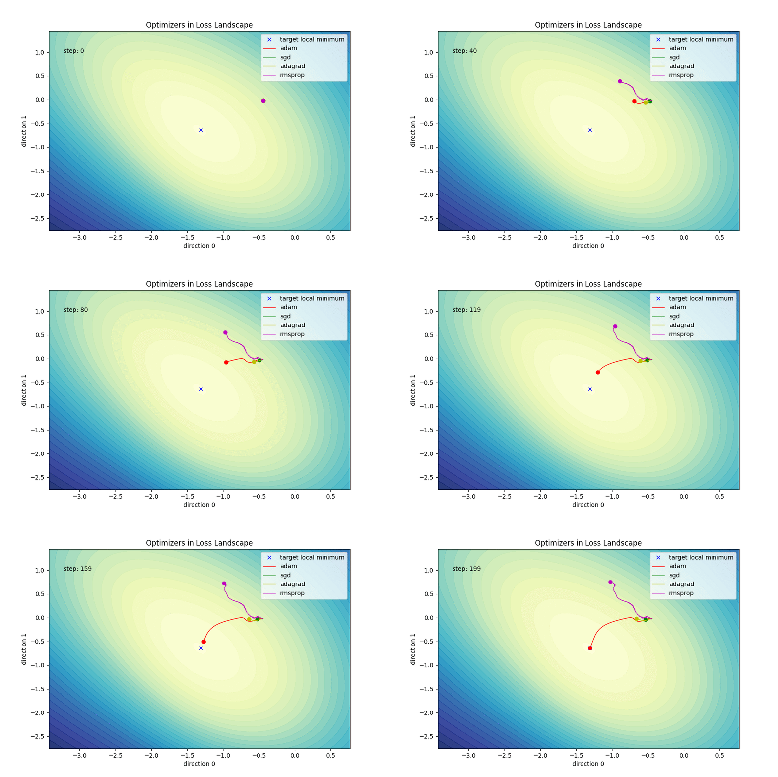
In this example, I have adam, sgd, adagrad, rmsprop initialized with the same parameters. The two figures below share the same 2 random directions but are centered around different local minima. The first figure centers around the one Adam finds, the second centers around the one RMSprop finds. Essentially, the planes are 2 parallel slices of the loss landscape.
The first figure shows that when centering on the end of Adam's path, it looks like RMSprop is going somewhere with larger loss value. But that is an illusion. If you inspect the loss values of RMSprop, it actually finds a local optimum that has a lower loss than Adam's.
Same 2 directions centering on Adam's path:
Same 2 directions centering on RMSprop's path:
This is a good reminder that the contours are just a 2D slice out of a very high-dimensional loss landscape, and the projections can't reflect the actual path.
However, we can see that the contours are convex no matter where it centers around in these 2 special cases. It more or less reflects that the optimizers shouldn't have a hard time finding a relatively good local minimum. To measure convexity more rigorously, the paper [1] mentioned a better method – using principal curvature, i.e. the eigenvalues of the Hessian. Check out the end of section 6 in the paper for more details.


