tokmaka1/ALKIA-X

ALKIA-X

ALKIA-X, the Adaptive and Localized Kernel Interpolation Algorithm with eXtrapolated reproducing kernel Hilbert space norm, is an algorithm to automatically approximate black-box functions. ALKIA-X ensures:

• A fast-to-evaluate approximating function;
• The guaranteed satisfaction of the desired bound on the approximation error;
• Well-conditioned computations;
• High level of parallelization.

We highlight the benefits of ALKIA-X by automatically approximating nonlinear model predictive control (MPC) schemes with closed-loop guarantees. Please refer to the [1] to cite this code.

[1] Abdullah Tokmak, Christian Fiedler, Melanie N. Zeilinger, Sebastian Trimpe, Johannes Köhler, "Automatic nonlinear MPC approximation with closed-loop guarantees," arXiv preprint arXiv:2312.10199, 2023.

Dependencies and setup

• Python
• CasADi and IPOPT for MPC problems
• anytree for the tree structure of the approximation
• concurrent.futures for parallel execution

Create a conda environment using the yml file:

conda env create -f ALKIAX.yml

Running ALKIA-X

You can run ALKIA-X as follows:

conda activate ALKIAX
taskset -c 1,2,3,4,5,6,7,8 python ALKIAX_main.py

This exact line will lead to a parallelization on CPU cores 1-8.

Toy example

2D sinusoide

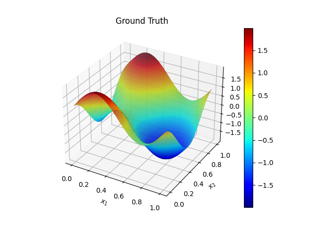
One of the toy examples is a two-dimensional sinusoide $f{:} [0,1]^2\subseteq\mathbb{R}^2\rightarrow \mathbb{R}$ $$f(x) = \sin(2\pi x_1)+ \cos(2\pi x_2),$$ with $x=[x_1,x_2]^\top.$ The following figure shows the ground truth function evaluated on $90\cdot 10^3$ equidistant inputs.

To execute the toy experiment, use the following hyperparameters in the ALKIAX_main.py file:

epsilon = 5e-3  # max allowed error
round_n_digits = 14  # rounding
gt_string = 'sine_2D'  # function to approximate
x_dim, y_dim = ground_truth_dimensions(gt_string)
number_of_head_nodes = 1  # no a-priori partitioning of the domain
p_min = 2  # minimum number of samples per sub-domain: (1+2**p_min)**n
cond_max = 1.15e8  # upper bound on the condition number of covariance matrices
C_ell = 0.8  # length scale parameter
kernel = matern_kernel(sigma=1, ell=C_ell, nu=3/2)
parallel = True  # for parallelization
max_storage_termination = np.infty  # no bound on the memory requirements

The epsilon-hyperparameter is the a priori guaranteed maximum approximation error. Decreasing that value will increase the approximation time (and vice versa). Save the resulting pickle file that contains the samples at the end of the ALKIAX_main.py file:

with open('C_root_sine_2D.pickle', 'wb') as handle:
    pickle.dump(C_root, handle, protocol=pickle.HIGHEST_PROTOCOL)

Then, execute the post processing by setting

gt_string = 'sine_2D'

in the ALKIAX_post.py file. There, the approximating functions are computed and the maximum error is determined. Moreover, the ground truth $f$ and the approximating function $h$ are plotted.

Ackley function

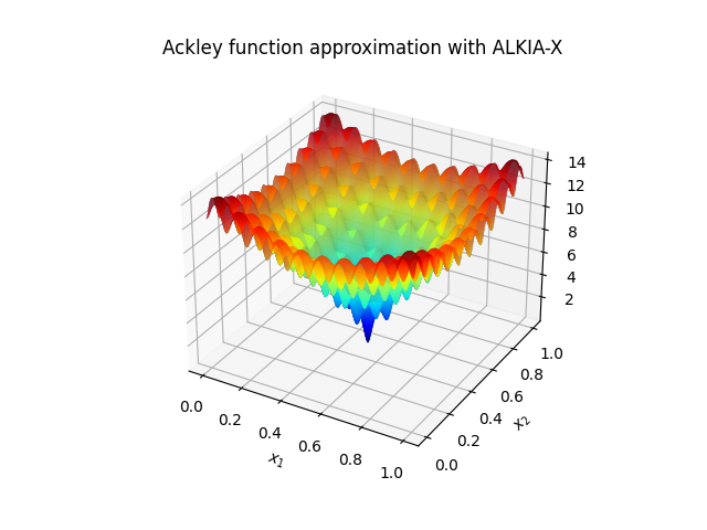
The Ackley function is given by $f{:} [0,1]^2\subseteq\mathbb{R}^2\rightarrow \mathbb{R}$ $$f(x) = -20 \exp\left(-0.2 \sqrt{\frac{x_1^2 + x_2^2}{2}}\right) - \exp\left(\frac{\cos(2\pi x_1) + \cos(2\pi x_2)}{2}\right) + 20 + e ,$$ with $x=[x_1,x_2]^\top.$ The following figure shows the ground truth function evaluated on $90\cdot 10^3$ equidistant inputs.

To execute the toy experiment, use the following hyperparameters in the ALKIAX_main.py file:

epsilon = 5e-2
round_n_digits = 14
gt_string = 'ackley'
x_dim, y_dim = ground_truth_dimensions(gt_string)
number_of_head_nodes = 16  # 16 a priori partitions
p_min = 2
cond_max = 1.15e8
C_ell = 0.8
kernel = matern_kernel(sigma=1, ell=C_ell, nu=3/2)
parallel = True
max_storage_termination = np.infty

Save the resulting pickle file that contains the samples at the end of the ALKIAX_main.py file:

with open('C_root_ackley.pickle', 'wb') as handle:
    pickle.dump(C_root, handle, protocol=pickle.HIGHEST_PROTOCOL)

Then, execute the post processing by setting

gt_string = 'ackley'

in the ALKIAX_post.py file. There, the approximating functions are computed and the maximum error is determined. Moreover, the ground truth $f$ and the approximating function $h$ are plotted.

Reproducing experiments of the paper

CSTR

To reproduce the approximation of the MPC scheme for the continious stirred tank reactor, use the following hyperparameters in the ALKIAX_main.py file:

epsilon = 5.1e-3
round_n_digits = 14
gt_string = 'CSTR_python'
x_dim, y_dim = ground_truth_dimensions(gt_string)
number_of_head_nodes = 5**2
p_min = 2
cond_max = 1.15e8
C_ell = 0.8
kernel = matern_kernel(sigma=1, ell=C_ell, nu=3/2)
parallel = True
max_storage_termination = np.infty  # no bound on the memory requirements

Save the resulting pickle file that contains the samples at the end of the ALKIAX_main.py file:

with open('C_root_CSTR.pickle', 'wb') as handle:
    pickle.dump(C_root, handle, protocol=pickle.HIGHEST_PROTOCOL)

You can also use the pre-trained pickle file in this repository (C_root_CSTR.pickle) and directly execute the post processing. For the post processing, set

gt_string = 'CSTR_python'

in the ALKIAX-post.py file. There, the approximating functions are computed and the maximum error is determined. Moreover, the MPC feedback law $f$ and the resulting sub-domain partitioning of ALKIA-X is plotted.

Cold atmospheric plasma

To reproduce the approximation of the MPC scheme for the cold atmospheric plasma device, use the following hyperparameters in the ALKIAX_main.py file:

epsilon = 1e-6
round_n_digits = 14
gt_string = 'plasma_python'
x_dim, y_dim = ground_truth_dimensions(gt_string)
number_of_head_nodes = 3**3
p_min = 2
cond_max = 3.4e7
C_ell = 0.8
kernel = matern_kernel(sigma=1, ell=C_ell, nu=3/2)
parallel = True
max_storage_termination = 75  # bound on the memory requirements, in MB

Save the resulting pickle file that contains the samples at the end of the ALKIAX_main.py file:

with open('C_root_plasma.pickle', 'wb') as handle:
    pickle.dump(C_root, handle, protocol=pickle.HIGHEST_PROTOCOL)

You can also use the pre-trained pickle file in this repository (C_root_CSTR.pickle) and directly execute the post processing. For the post processing, set

gt_string = 'plasma_python'

in the ALKIAX-post.py file. First, the closed-loop trajectories of the MPC are determined. Then, the approximate MPC using ALKIA-X is computed and the closed-loop trajectories of the approximate MPC are determined. Moreover, the online evaluation of the MPC and the approximate MPC are assessed. Before plotting the closed-loop trajectories, the maximum input error between the MPC and the approximate MPC on the closed-loop state trajectory of the approximate MPC is calculated.