For instructions on how to setup and run this project go to the starter code section.
The write-up below is also available here as a blog post.
For artificial intelligence (AI) to reach its full potential, AI systems need to interact safely and efficiently with humans, as well as other agents. There are already environments where this happens on a daily basis, such as the stock market. And there are future applications that will rely on productive agent-human interactions, such as self-driving cars and other autonomous vehicles.
One step along this path is to train AI agents to interact with other agents in both cooperative and competitive settings. Reinforcement learning (RL) is a subfield of AI that's shown promise. However, thus far, much of RL's success has been in single agent domains, where building models that predict the behavior of other actors is unnecessary. As a result, traditional RL approaches (such as Q-Learning) are not well-suited for the complexity that accompanies environments where multiple agents are continuously interacting and evolving their policies.
The goal of this project is to train two RL agents to play tennis. As in real tennis, the goal of each player is to keep the ball in play. And, when you have two equally matched opponents, you tend to see fairly long exchanges where the players hit the ball back and forth over the net.
We'll work with an environment that is similar, but not identical to the Tennis environment on the Unity ML-Agents GitHub page.
In this environment, two agents control rackets to bounce a ball over a net. If an agent hits the ball over the net, it receives a reward of +0.1. If an agent lets a ball hit the ground or hits the ball out of bounds, it receives a reward of -0.01. Thus, the goal of each agent is to keep the ball in play.
The observation space consists of 8 variables corresponding to the position and velocity of the ball and racket. Each agent receives its own, local observation. Two continuous actions are available, corresponding to moves toward (or away from) the net, and jumping.
The task is episodic, and in order to solve the environment, your agents must get an average score of +0.5 (over 100 consecutive episodes, after taking the maximum over both agents). Specifically,
- After each episode, we add up the rewards that each agent received (without discounting), to get a score for each agent. This yields 2 (potentially different) scores. We then take the maximum of these 2 scores.
- This yields a single score for each episode.
The environment is considered solved when the average (over 100 episodes) of those scores is at least +0.5.
Here are the high-level steps taken in building an agent that solves this environment.
- Establish performance baseline using a random action policy.
- Select an appropriate algorithm and begin implementing it.
- Run experiments, make revisions, and retrain the agent until the performance threshold is reached.
WARNING: I ultimately reached a good solution; however, the results were not consistent. My "best" results were only reproducible if I reran the model numerous times (>10). If you just run the model once (or even 3-5 times), it might not converge. And, during the initial implementation, I ran the model at least 30 times while searching for a reliable set of hyperparameters. If you want to experiment with different approaches, I strongly recommend implementing a more systematic approach such as grid search (which I did not do, but wish I had).
Before building agents that learn, I started by testing ones that select actions (uniformly) at random at each time step.
Running the random agents a few times resulted in scores from 0 to 0.02. Obviously, if these agents need to achieve an average score of 0.5 over 100 consecutive episodes, then choosing actions at random won't work. However, when you watch the agents acting randomly, it becomes clear that these types of sporadic actions can be useful early in the training process. That is, they can help the agents explore the action space to find some signal of good vs. bad actions. This insight will come into play later when we implement the Ornstein-Uhlenbeck process and epsilon noise decay.
To get started, there are a few high-level architecture decisions we need to make. First, we need to determine which types of algorithms are most suitable for the Tennis environment.
There are two key differences in the Tennis environment compared to the 'Navigation' environment from two projects ago:
- Multiple agents — The Tennis environment has 2 different agents, whereas the Navigation project had only a single agent.
- Continuous action space — The action space is now continuous, which allows each agent to execute more complex and precise movements. Even though each tennis agent can only move forward, backward, or jump, there's an unlimited range of possible action values that control these movements. Whereas, the agent in the Navigation project was limited to four discrete actions: left, right, forward, backward.
Given the additional complexity of this environment, the value-based method we used for the Navigation project is not suitable — i.e., the Deep Q-Network (DQN) algorithm. Most importantly, we need an algorithm that allows the tennis agent to utilize its full range and power of movement. For this, we'll need to explore a different class of algorithms called policy-based methods.
Here are some advantages of policy-based methods:
- Continuous action spaces — Policy-based methods are well-suited for continuous action spaces.
- Stochastic policies — Both value-based and policy-based methods can learn deterministic policies. However, policy-based methods can also learn true stochastic policies.
- Simplicity — Policy-based methods directly learn the optimal policy, without having to maintain a separate value function estimate. With value-based methods, the agent uses its experience with the environment to maintain an estimate of the optimal action-value function, from which an optimal policy is derived. This intermediate step requires the storage of lots of additional data since you need to account for all possible action values. Even if you discretize the action space, the number of possible actions can get quite large. And, using DQN to determine the action that maximizes the action-value function within a continuous or high-dimensional space requires a complex optimization process at every timestep.
The original DDPG algorithm from which I extended to create the MADDPG version, is outlined in this paper, Continuous Control with Deep Reinforcement Learning, by researchers at Google Deepmind. In this paper, the authors present "a model-free, off-policy actor-critic algorithm using deep function approximators that can learn policies in high-dimensional, continuous action spaces." They highlight that DDPG can be viewed as an extension of Deep Q-learning to continuous tasks.
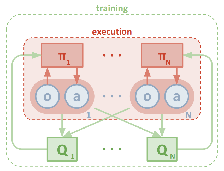
For the DDPG foundation, I used this vanilla, single-agent DDPG as a template. Then, to make this algorithm suitable for the multiple competitive agents in the Tennis environment, I implemented components discussed in this paper, Multi-Agent Actor-Critic for Mixed Cooperative-Competitive Environments, by Lowe and Wu, along with other researchers from OpenAI, UC Berkeley, and McGill University. Most notable, I implemented their variation of the actor-critic method (see Figure 1), which I discuss in the following section.
Lastly, I further experimented with components of the DDPG algorithm based on other concepts covered in Udacity's classroom and lessons. My implementation of this algorithm (including various customizations) are discussed below.
Figure 1: Multi-agent decentralized actor with centralized critic (Lowe and Wu et al).
Actor-critic methods leverage the strengths of both policy-based and value-based methods.
Using a policy-based approach, the agent (actor) learns how to act by directly estimating the optimal policy and maximizing reward through gradient ascent. Meanwhile, employing a value-based approach, the agent (critic) learns how to estimate the value (i.e., the future cumulative reward) of different state-action pairs. Actor-critic methods combine these two approaches in order to accelerate the learning process. Actor-critic agents are also more stable than value-based agents, while requiring fewer training samples than policy-based agents.
What makes this implementation unique is the decentralized actor with centralized critic approach from the paper by Lowe and Wu. Whereas traditional actor-critic methods have a separate critic for each agent, this approach utilizes a single critic that receives as input the actions and state observations from all agents. This extra information makes training easier and allows for centralized training with decentralized execution. Each agent still takes actions based on its own unique observations of the environment.
You can find the actor-critic logic implemented as part of the Agent() class here in maddpg_agent.py of the source code. The actor-critic models can be found via their respective Actor() and Critic() classes here in models.py.
Note: As we did with Double Q-Learning in the last project, we're again leveraging local and target networks to improve stability. This is where one set of parameters w is used to select the best action, and another set of parameters w' is used to evaluate that action. In this project, local and target networks are implemented separately for both the actor and the critic.
# Actor Network (w/ Target Network)
self.actor_local = Actor(state_size, action_size, random_seed).to(device)
self.actor_target = Actor(state_size, action_size, random_seed).to(device)
self.actor_optimizer = optim.Adam(self.actor_local.parameters(), lr=LR_ACTOR)

# Critic Network (w/ Target Network)
self.critic_local = Critic(state_size, action_size, random_seed).to(device)
self.critic_target = Critic(state_size, action_size, random_seed).to(device)
self.critic_optimizer = optim.Adam(self.critic_local.parameters(), lr=LR_CRITIC, weight_decay=WEIGHT_DECAY)One challenge is choosing which action to take while the agent is still learning the optimal policy. Should the agent choose an action based on the rewards observed thus far? Or, should the agent try a new action in hopes of earning a higher reward? This is known as the exploration vs. exploitation dilemma.
In the Navigation project, I addressed this by implementing an 𝛆-greedy algorithm. This algorithm allows the agent to systematically manage the exploration vs. exploitation trade-off. The agent "explores" by picking a random action with some probability epsilon 𝛜. Meanwhile, the agent continues to "exploit" its knowledge of the environment by choosing actions based on the deterministic policy with probability (1-𝛜).
However, this approach won't work for controlling the tennis agents. The reason is that the actions are no longer a discrete set of simple directions (i.e., up, down, left, right). The actions driving the movement of the arm are forces with different magnitudes and directions. If we base our exploration mechanism on random uniform sampling, the direction actions would have a mean of zero, in turn canceling each other out. This can cause the system to oscillate without making much progress.
Instead, we'll use the Ornstein-Uhlenbeck process, as suggested in the previously mentioned paper by Google DeepMind (see bottom of page 4). The Ornstein-Uhlenbeck process adds a certain amount of noise to the action values at each timestep. This noise is correlated to previous noise and therefore tends to stay in the same direction for longer durations without canceling itself out. This allows the agent to maintain velocity and explore the action space with more continuity.
You can find the Ornstein-Uhlenbeck process implemented here in the OUNoise class in maddpg_agent.py of the source code.
In total, there are five hyperparameters related to this noise process.
The Ornstein-Uhlenbeck process itself has three hyperparameters that determine the noise characteristics and magnitude:
- mu: the long-running mean
- theta: the speed of mean reversion
- sigma: the volatility parameter
Of these, I only tuned sigma. After running a few experiments, I reduced sigma from 0.3 to 0.2. The reduced noise volatility seemed to help the model converge.
Notice also there's an epsilon parameter used to decay the noise level over time. This decay mechanism ensures that more noise is introduced earlier in the training process (i.e., higher exploration), and the noise decreases over time as the agent gains more experience (i.e., higher exploitation). The starting value for epsilon and its decay rate are two hyperparameters that were tuned during experimentation.
You can find the epsilon decay process implemented here in the Agent.act() method in maddpg_agent.py of the source code. While the epsilon decay is performed here as part of the learning step.
The final noise parameters were set as follows:
OU_SIGMA = 0.2          # Ornstein-Uhlenbeck noise parameter, volatility
OU_THETA = 0.15          # Ornstein-Uhlenbeck noise parameter, speed of mean reversion
EPS_START = 5.0         # initial value for epsilon in noise decay process in Agent.act()
EPS_EP_END = 300        # episode to end the noise decay process
EPS_FINAL = 0           # final value for epsilon after decay
IMPORTANT NOTE: Notice that the EPS_START parameter is set at 5.0. For dozens of experiments, I had this parameter set to 1.0, as I had in previous projects. But, I had a difficult time getting the model to converge, and if it did, it converged very slowly (>1500 episodes). After much trial and error, I realized that the agents had some difficulty discovering signal early in the process (i.e., most episode scores equaled zero). By boosting the noise output from the Ornstein-Uhlenbeck (OU) process, it encouraged aggressive exploration of the action space and therefore improved the chances that signal would be detected (i.e., making contact with the ball). This extra signal seemed to improve learning later in training once the noise decayed to zero.
In the first few versions of my implementation, the agent only performed a single learning iteration per episode. Although the best model had this setting, this seemed to be a stroke of luck. In general, I found that performing multiple learning passes per episode yielded faster convergence and higher scores. This did make training slower, but it was a worthwhile trade-off. In the end, I implemented an interval in which the learning step is performed every episode. As part of each learning step, the algorithm then samples experiences from the buffer and runs the Agent.learn() method 10 times.
LEARN_EVERY = 1         # learning interval (no. of episodes)
LEARN_NUM = 5           # number of passes per learning step
You can find the learning interval implemented here in the Agent.step() method in maddpg_agent.py of the source code.
In early versions of my implementation, I had trouble getting my agent to learn. Or, rather, it would start to learn but then become very unstable and either plateau or collapse.
I suspect that one of the causes was outsized gradients. Unfortunately, I couldn't find an easy way to investigate this, although I'm sure there's some way of doing this in PyTorch. Absent this investigation, I hypothesize that many of the weights from my critic model were becoming quite large after just 50-100 episodes of training. And since I was running the learning process multiple times per episode, it only made the problem worse.
The issue of exploding gradients is described in layman's terms in this post by Jason Brownlee. Essentially, each layer of your net amplifies the gradient it receives. This becomes a problem when the lower layers of the network accumulate huge gradients, making their respective weight updates too large to allow the model to learn anything.
To combat this, I implemented gradient clipping using the torch.nn.utils.clip_grad_norm_ function. I set the function to "clip" the norm of the gradients at 1, therefore placing an upper limit on the size of the parameter updates, and preventing them from growing exponentially. Once this change was implemented, along with batch normalization (discussed in the next section), my model became much more stable and my agent started learning at a much faster rate.
You can find gradient clipping implemented here in the "update critic" section of the Agent.learn() method, within ddpg_agent.py of the source code.
Note that this function is applied after the backward pass, but before the optimization step.
# Compute critic loss
Q_expected = self.critic_local(states, actions)
critic_loss = F.mse_loss(Q_expected, Q_targets)
# Minimize the loss
self.critic_optimizer.zero_grad()
critic_loss.backward()
torch.nn.utils.clip_grad_norm_(self.critic_local.parameters(), 1)
self.critic_optimizer.step()
Experience replay allows the RL agent to learn from past experience.
As with the previous project, the algorithm employs a replay buffer to gather experiences. Experiences are stored in a single replay buffer as each agent interacts with the environment. These experiences are then utilized by the central critic, therefore allowing the agents to learn from each others' experiences.
The replay buffer contains a collection of experience tuples with the state, action, reward, and next state (s, a, r, s'). The critic samples from this buffer as part of the learning step. Experiences are sampled randomly, so that the data is uncorrelated. This prevents action values from oscillating or diverging catastrophically, since a naive algorithm could otherwise become biased by correlations between sequential experience tuples.
Also, experience replay improves learning through repetition. By doing multiple passes over the data, our agents have multiple opportunities to learn from a single experience tuple. This is particularly useful for state-action pairs that occur infrequently within the environment.
The implementation of the replay buffer can be found here in the maddpg_agent.py file of the source code.
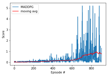
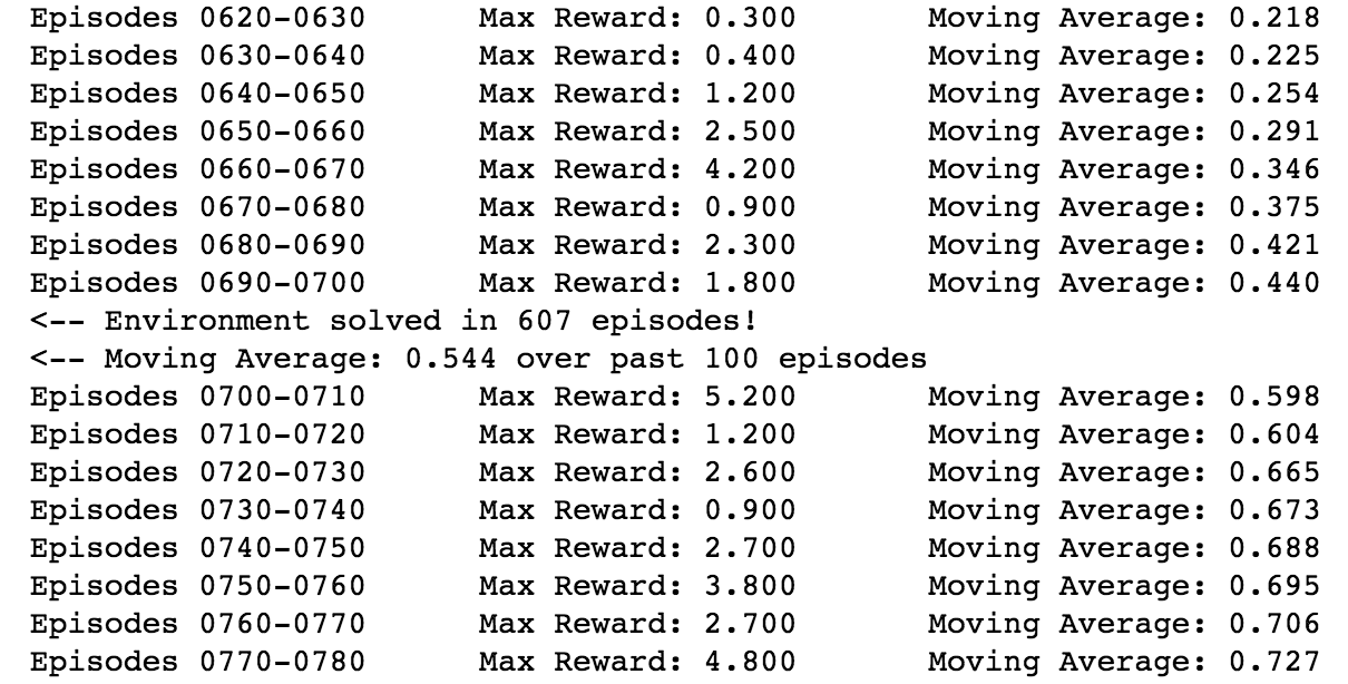
Once all of the above components were in place, the agents were able to solve the Tennis environment. Again, the performance goal is an average reward of at least +0.5 over 100 episodes, taking the best score from either agent for a given episode.
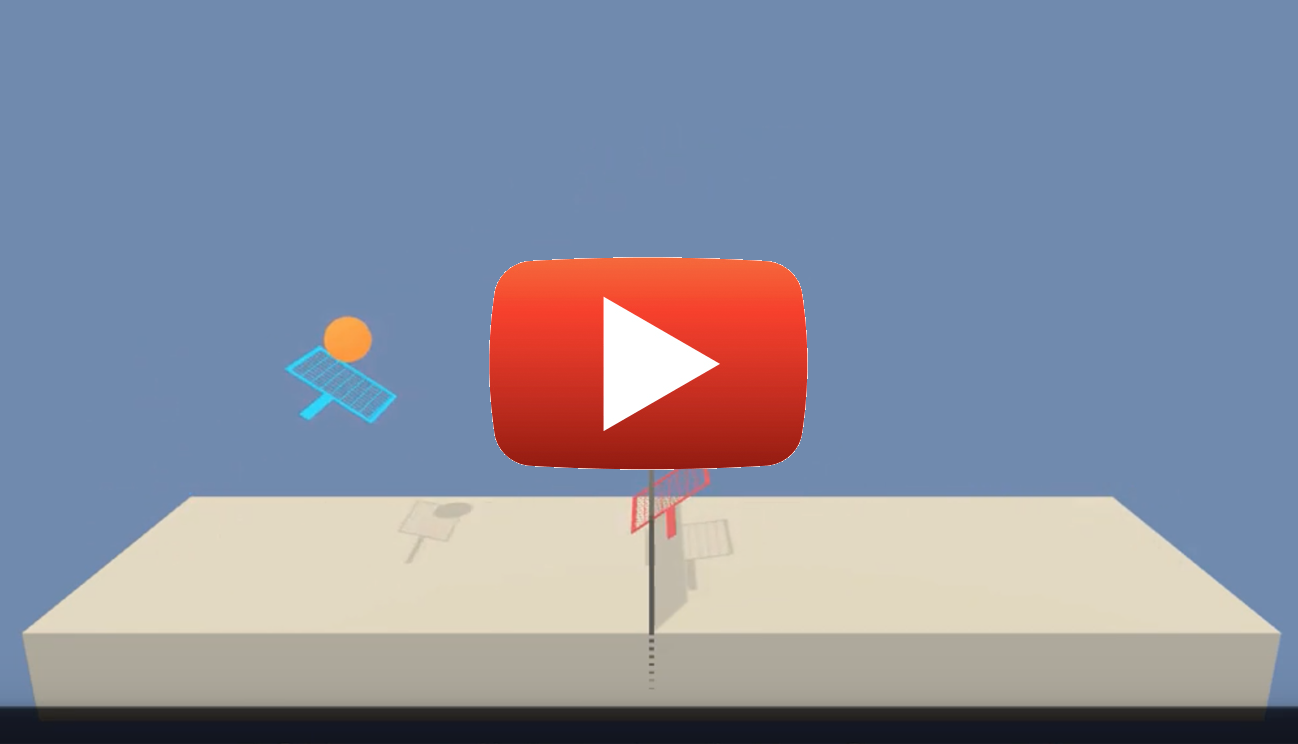
Here is a video showing the trained agents playing a few points.
The graph below shows the final training results. The best-performing agents were able to solve the environment in 607 episodes, with a top score of 5.2 and a top moving average of 0.927. The complete set of results and steps can be found in this notebook.
- Address stability issues to produce more consistent results — My "best" results are only reproducible if you run the model numerous times. If you just run it once (or even 3-5 times) the model might not converge. I ran the model at least 30 while searching for a good set of hyperparameters, so perhaps implementing a more systemic approach such as grid search would help. Otherwise, more research is needed to find a more stable algorithm, or to make changes to the current DDPG algorithm.
- Add prioritized experience replay — Rather than selecting experience tuples randomly, prioritized replay selects experiences based on a priority value that is correlated with the magnitude of error. This can improve learning by increasing the probability that rare or important experience vectors are sampled.
- Batch Normalization — I did not use batch normalization on this project, but I probably should have. I've used batch normalization many times in the past when building convolutional neural networks (CNN), in order to squash pixel values. But, it didn't occur to me that it would be to this project. This is an aspect of this Google DeepMind paper that has proved tremendously useful in my implementation of other projects.
- Similar to the exploding gradient issue mentioned above, running computations on large input values and model parameters can inhibit learning. Batch normalization addresses this problem by scaling the features to be within the same range throughout the model and across different environments and units. In additional to normalizing each dimension to have unit mean and variance, the range of values is often much smaller, typically between 0 and 1.
- You can find batch normalization implemented here for the actor, and here for the critic, within
model.pyof the source code of my previous project. These greatly improved model performance.
If you want to run this project yourself, the project starter code can be found below or here within Udacity's source repo for this project.
-
Download the environment from one of the links below. You need only select the environment that matches your operating system:
- Linux: click here
- Mac OSX: click here
- Windows (32-bit): click here
- Windows (64-bit): click here
(For Windows users) Check out this link if you need help with determining if your computer is running a 32-bit version or 64-bit version of the Windows operating system.
(For AWS) If you'd like to train the agent on AWS (and have not enabled a virtual screen), then please use this link to obtain the "headless" version of the environment. You will not be able to watch the agent without enabling a virtual screen, but you will be able to train the agent. (To watch the agent, you should follow the instructions to enable a virtual screen, and then download the environment for the Linux operating system above.)
-
Place the file in the DRLND GitHub repository, in the
p3_collab-compet/folder, and unzip (or decompress) the file.
You can run the code using the following command in your terminal:
You can also follow the instructions in Tennis.ipynb.
After you have successfully completed the project, you might like to solve the more difficult Soccer environment.
In this environment, the goal is to train a team of agents to play soccer.
You can read more about this environment in the ML-Agents GitHub here. To solve this harder task, you'll need to download a new Unity environment. (Note: Udacity students should not submit a project with this new environment.)
You need only select the environment that matches your operating system:
- Linux: click here
- Mac OSX: click here
- Windows (32-bit): click here
- Windows (64-bit): click here
Then, place the file in the p3_collab-compet/ folder in the DRLND GitHub repository, and unzip (or decompress) the file. Next, open Soccer.ipynb and follow the instructions to learn how to use the Python API to control the agent.
(For AWS) If you'd like to train the agents on AWS (and have not enabled a virtual screen), then please use this link to obtain the "headless" version of the environment. You will not be able to watch the agents without enabling a virtual screen, but you will be able to train the agents. (To watch the agents, you should follow the instructions to enable a virtual screen, and then download the environment for the Linux operating system above.)
