Analysis notes for "National and International Dimensions of HIV-1 Sequence Clusters in a Northern California Clinical Cohort"
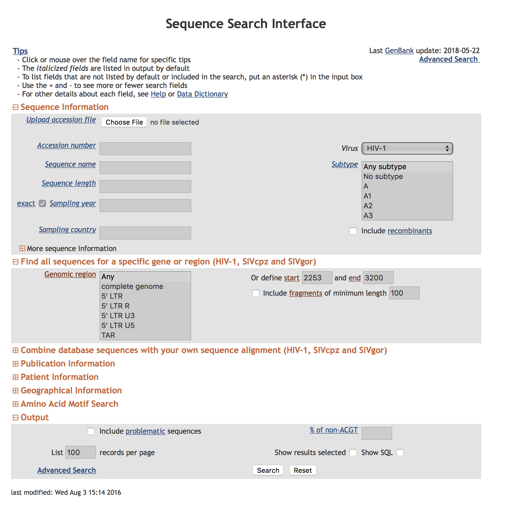
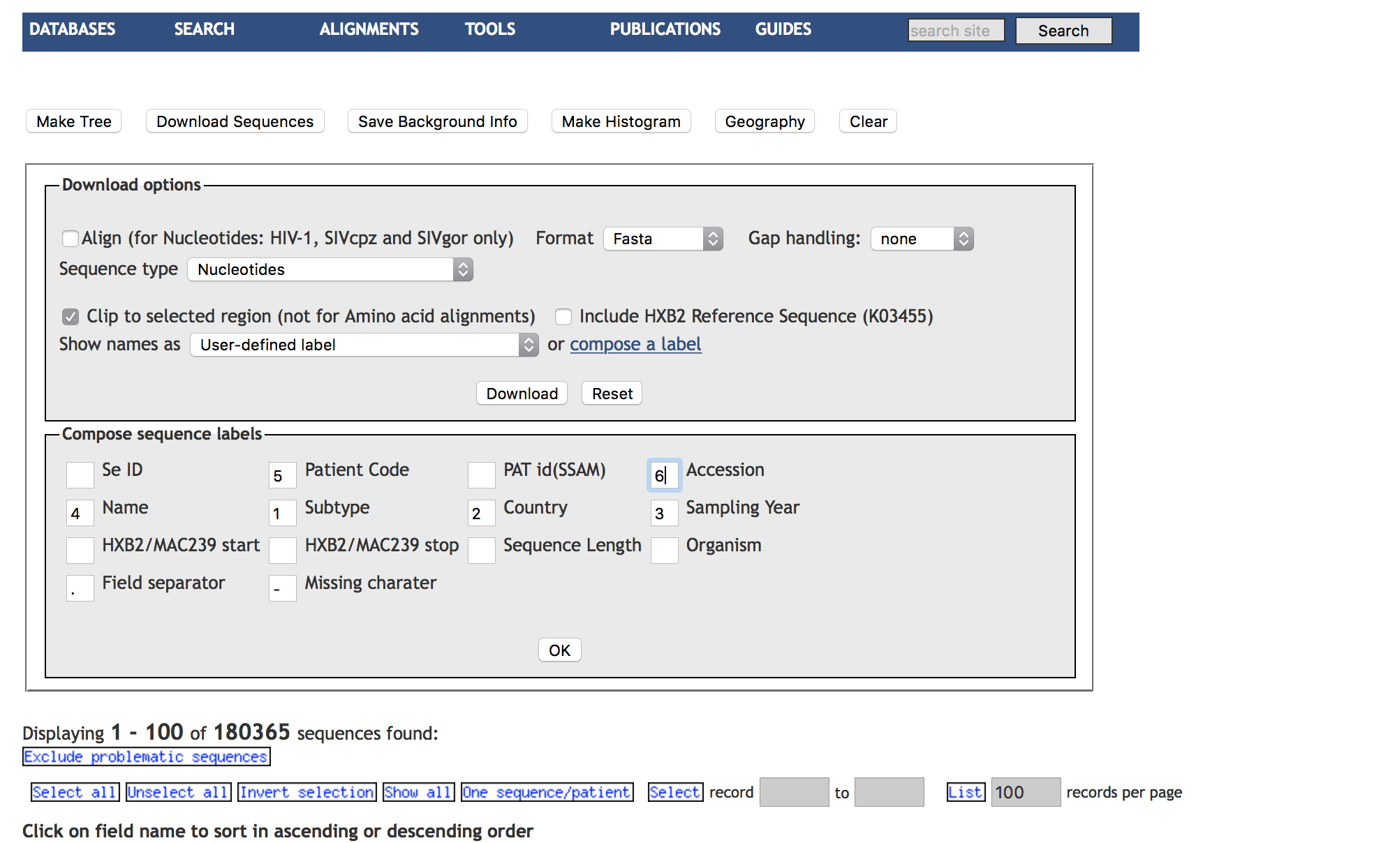
We searched the HIV LANL database to include all HIV-1 sequencies covering all of PR and the first 200 (or more) aminoacids of RT. We excluded problematic sequences (which is the default setting) and selected one sequence per individual for download. We composed a custom label for sequence downloads. See attached screenshots.
The resulting file contained 140464 sequences and can be found in data/raw_reference.fas
The standard workflow for preparing the LANL file for consumption by HIV-TRACE is
Step 1. Align all database sequences to the same reference as will be used for KP data using bealign
By convention we use the HXB2_prrt reference sequence; this is the HBX2 strain's PR and RT. We also specify an HIV-specific scoring matrix (HIV_BETWEEN_F), from this Nickle et al paper. The command to align sequences is as follows (adjust path names accordingly, assumes bealign has been installed); this step takea about 25 minutes on a MacBook Pro (running in multi-threaded mode).
$bealign -r HXB2_prrt -m HIV_BETWEEN_F data/raw_reference.fas data/reference.bam
Use the command (which is a part of the BioExt package):
$bam2msa data/reference.bam data/reference-aligned.fas
We repeat the same steps for the data/KP-naive.fas dataset with the resulting files data/kp-mapped.bam and data/kp-aligned.fas. When invoking bealign on the KP-naive.fas file.
$bealign -r HXB2_prrt -m HIV_BETWEEN_F data/kp_naive.fas data/kp-mapped.bam
$bam2msa data/kp-mapped.bam data/kp-aligned.fas
Because some of the database sequences include those deposited by Stanford, we filter the reference database to exclude all the blacklisted sequences contained in the file data/stanford-accessions.csv (second column) via the following command
$python3 scripts/filter-accession-numbers-fas.py -i data/stanford-accessions.csv
-f data/reference-aligned.fas > data/reference-aligned-filtered.fas
The resulting file with "clean" accession numbers is written to data/reference-aligned-filtered.fas and excludes 1404 sequences from the original download. The total number of sequences in this file is 139060 sequences.
Next, we perform the combined KP and LANL HIV-TRACE analysis.
[Step 1] Computing pairwise TN93 distances using the tn93 tool.
[Step 2] Inferring the transmission network using hivnetworkcsv
[Step 3] Incorporating external attributes for nodes from the TSV file
[Step 4] Summarizing the network using ancillary scripts
[Step 5] Visualizing the results using hivtrace-viz
Our suggested way to handle ambiguous data is as follows: resolve all two-way ambiguities to match their possible single character states, average all other ambiguites, ignore positions where either sequence has a gap, and for ambiguity rich sequences (>5% of bases are ambiguous), we average all resolutions.
Other options provided to the analysis request that only sequences that have 500 or more aligned bases be compared and only distances of 1.5% or less be output to the CSV file.
We compute the pairwise distances using the TN93 tool.
Compute pairwise distsnces between all pairs of KP sequences and write those ≤1.5% to
results/kp-distances.csv
$tn93 -a RYWSMK -g 0.05 -l 500 -t 0.015 -o results/kp-distances.csv data/kp-aligned.fas
Overall run metrics are printed to the console (see below); in particular, 4151 pairs of sequences were linked at 1.5% or less genetic distance.
	"Actual comparisons performed" :10362628,
	"Comparisons accounting for copy numbers " :1.03626e+07,
	"Total comparisons possible" : 10362628,
	"Links found" : 4151,
	"Maximum distance" : 0.164805,
	"Sequences" : 4553,
	"Mean distance" : 0.0611479
Compute pairwise distsnces between all pairs of (KP, LANL) sequences and write those ≤1.5% to
results/kp-lanl.csv
$tn93 -a RYWSMK -g 0.05 -l 500 -t 0.015 -o results/kp-lanl.csv
-s data/reference-aligned-filtered.fas data/kp-aligned.fas
This step takes approximately 3 minutes on a MacBook Pro (running in multithreaded mode)
Overall run metrics are printed to the console (see below), in particular, 9970 pairs of (KP, LANL) sequences were linked at 1.5% or less genetic distance.
"Actual comparisons performed" :633140180,
	"Comparisons accounting for copy numbers " :6.3314e+08,
	"Total comparisons possible" : 633140180,
	"Links found" : 9970,
	"Maximum distance" : 0.427186,
	"Sequences in first file" : 4553,
	"Sequences in second file" : 139060,
	"Mean distance" : 0.085368,
Compute pairwise distsnces between all pairs of LANL sequences and write those ≤1.0% to
results/lanl-lanl.csv
This step takes approximately an hour on a MacBook Pro (running in multithreaded mode), since it performs close to 10 billion pairwise distance calculations.
$tn93 -a RYWSMK -g 0.05 -l 500 -t 0.01 -o results/lanl-lanl.csv
data/reference-aligned-filtered.fas
Overall run metrics are printed to the console (see below), in particular, 588391 pairs of LANL sequences were linked at 1.0% or less genetic distance.
	"Actual comparisons performed" :9668772270,
	"Comparisons accounting for copy numbers " :9.66877e+09,
	"Total comparisons possible" : 9668772270,
	"Links found" : 588391,
	"Maximum distance" : 0.682983,
	"Sequences" : 139060,
	"Mean distance" : 0.0976466,
We will use hivnetworkcsv, which is a part of HIV-TRACE package, to infer the transmission network.
The recommended set of options, which use edge filtering to consider all network triangles (A connected to B connected to C connected to A), and uses a phylogenetic test to remove one of the traingle edges if possible, and mark sequences that are in clusters with HXB2 as potential contaminants (in your case, because you have old sequences these clusters are probably real). Please note that the data/hxb2.txt file lists the name of the reference sequence used by bealign during the mapping stage; if you change the reference sequence there, you should also update this file.
We will also be excluding those clusters which contain LANL sequences (i.e. no KP isolates). In order to do so, we need to prepare a file that lists all KP sequence IDs (the whitelist); this can be done using the following command
awk '/^\>/ {print substr($0,2);}' data/kp-aligned.fas > data/kp-ids.txt
The following command takes about 8-10 hours to run on a MacBook Pro, with >99% of the time consumed by edge filtering.
$ hivnetworkcsv -t 0.015 -j -i results/kp-distances.csv -i results/kp-lanl.csv
-i results/lanl-lanl.csv -f plain -f plain -f plain -k data/kp-ids.txt
-s data/kp-aligned.fas -s data/reference-aligned-filtered.fas
-s data/reference-aligned-filtered.fas -n remove > results/network.json
The program will write progress messages to the screen along the lines of
Included 405852 edges after applying node list filtering
Running edge filtering on 278 clusters with 3 or more edges
Filtering a set of 5946 edges (273/278 clusters). Pass 0, 32768 triangles, 1433 filtered edges
...
...
conclude with the summary of actions performed,
Edge filtering identified 118231 edges for removal
Edge filtering removed 118231 edges
Fitting the degree distribution to various densities
and write the resulting network as a JSON file to results/network.json.
To annotate network with attributes that can be viewed and interacted with using hivnetwork-viz, and summarized with ancillary scripts, we will use a variety of simple Python scripts to extract sequence attributes from sequence names and CSV/TSV files.
The first order of business is to extract country and isolation year from LANL sequences. This is done in two steps
1). Extract year and country of isolation and the subtype from . delimited sequence names, like C.IN.1993.93IN101.IN101.AB023804
2). Take advantage of additional information about the 9397 sequences from [PMID 15567861] (https://www.ncbi.nlm.nih.gov/pubmed/15567861), that are marked as having 'unknown' country in LANL, but are all 'US' based isolates (based on the provenance of the lab and personal communication from study authors).
$python3 scripts/extract-lanl-annotations.py
-d results/kp-lanl.csv -d results/lanl-lanl.csv
-i data/PMID-15567861-accessions.txt 1 'US' > data/lanl-annotations.tsv
The resulting file data/lanl-annotations.tsv looks like
ID	Country	IsolateYear	Subtype
B.FR.1983.IIIB_LAI.LAI.A04321	FR	1983	B
B.JP.-.KI_560.KI_560.AB873942	JP	-	B
01_AE.VN.2009.09HT0038PRRT.-.AB895317	VN	2009	01_AE
B.US.-.33C.-.AF072959	US	-	B
B.IT.-.163.-.AF252022	IT	-	B...
Next, we "inject" attributes into the network JSON file using a series of calls to a Python script scripts/inject-attributes.py. There is a shell script scripts/annotate-network.sh which automates the repeated invokation of scripts/inject-attributes.py to store Year and Country into the network JSON file, as well as annotate each node with whether or not it came from KP or LANL ('Source'). We also annotate LANL sequences by subtype
sh scripts/annotate-network.sh results/network
Load the resulting json into the visualization into veg.github.io/hivtrace-viz/plain.html, using the FILE menu, to view the networks .JSON file.
We have created an ObservableHQ notebook which pulls the network.json file from Dropbox and performs live analyis and figure generation of some of the descriptive text in the manuscript.
A part of the analysis involves extracting indivudal clusters from the network, which can be done with the help of scripts/extract-cluster.py. For example, to extract the list of sequence IDs to cluster 2 (the large subtype B cluster to), we use
$scripts/extract-cluster.py -j results/network.json -c 2
which outputs a long list sequence names to stdout
B.ES.-.34_00.-.AY316019
B.AU.2007.99619831.99619831.KC238301
B.CN.2008.2008_ZheJiang_QZ08ZJ180_MTB.08ZJ180.KJ614180
B.-.2002.02_126855.-.EU608080
B.CN.2011.LS3349.LS3349.KT379174
B.JP.2010.E10-50910963-1.E10-50910963.AB866110
B.CN.2008.SQ9_4.-.GU345702
30155
...
This script can also extract sequences associated with clustered sequences, if it provided with the corresponding FASTA files, e.g.,
$python3 scripts/extract-cluster.py -j results/network.json -c 2
-f data/kp-aligned.fas -f data/reference-aligned.fas
In order to subsample larger clusters to enable faster phylogenetic analyses, please use the scripts/thin-cluster.sh shell script, which relies on subset-cluster.py, scripts/extract-cluster.py, TN93, and FASTTree (assumed to be installed and availabe via PATH environment variable)
Use as follows to extract cluster 287 to directory clusters/cluster287-AE and thin in down to 200 sequences, including all NCC sequences
$sh scripts/thin-cluster.sh cluster287-AE 287 200
The resulting direcoty will contain the following files:
ls -l clusters/cluster287-AE/
total 19352
-rw-r--r--@ 1 sergei  staff  4170544 Dec 12 15:13 dense-clusters.json
-rw-r--r--@ 1 sergei  staff       81 Dec 12 15:13 ncc.txt
-rw-r--r--@ 1 sergei  staff  5175701 Dec 12 15:13 sequences.fas
-rw-r--r--@ 1 sergei  staff   331008 Dec 12 15:13 subset-200.fas
-rw-r--r--@ 1 sergei  staff    11566 Dec 12 15:13 subset-200.tree
| File | Contents |
|---|---|
| dense-clusters.json | A JSON files with all subclusters at 0.5% or less |
| ncc.txt | The list of NCC sequence IDs in the cluster |
| sequences.fas | FASTA sequences for all the members of this cluster |
| sequences-200.fas | FASTA sequences for the subsampled cluster |
| sequences-200.tree | FastTree tree in Newick format, based on the subsampled cluster |

