INLAutils

A package containing utility functions for the R-INLA package.

There's a fair bit of overlap with inlabru.

Installation

To install, first install INLA.

install.packages("INLA", repos="https://www.math.ntnu.no/inla/R/stable")

then install INLAutils

# From github
library(devtools)
install_github('timcdlucas/INLAutils')

# Load packages
library(INLA)
library(INLAutils)

Unfortunately, CRAN have now decided that as INLA is not on CRAN, INLAutils cannot be on CRAN either (a totally reasonable position).

Overview

Plotting

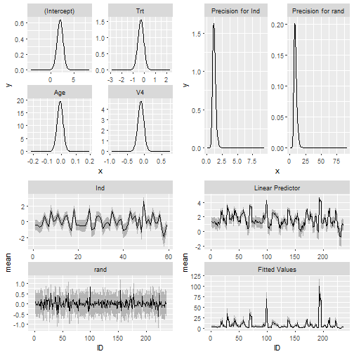
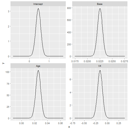
I find the the plot function in INLA annoying and I like ggplot2. So INLAutils provides an autoplot method for INLA objects.

      data(Epil)
      ##Define the model
      formula = y ~ Trt + Age + V4 +
               f(Ind, model="iid") + f(rand,model="iid")
      result = inla(formula, family="poisson", data = Epil, control.predictor = list(compute = TRUE))
     
      autoplot(result)

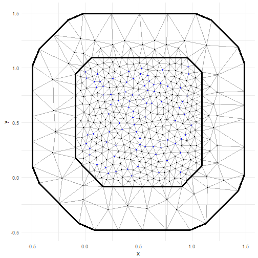
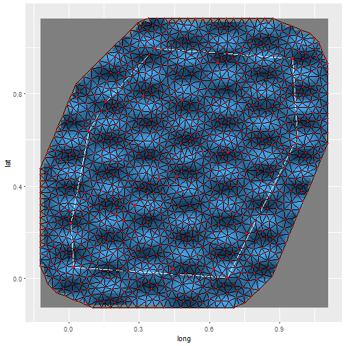
There is an autoplot method for INLA SPDE meshes.

    m = 100
    points = matrix(runif(m * 2), m, 2)
    mesh = inla.mesh.create.helper(
      points = points,
      cutoff = 0.05,
      offset = c(0.1, 0.4),
      max.edge = c(0.05, 0.5))
    
    autoplot(mesh)

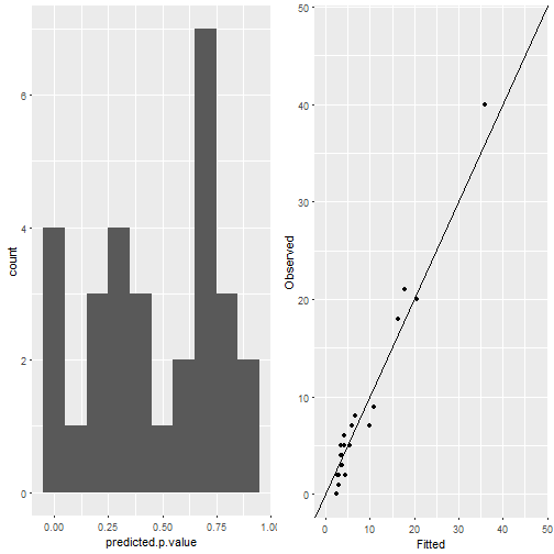
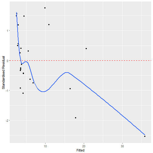
There are functions for plotting more diagnostic plots.

 data(Epil)
 observed <- Epil[1:30, 'y']
 Epil <- rbind(Epil, Epil[1:30, ])
 Epil[1:30, 'y'] <- NA
 ## make centered covariates
 formula = y ~ Trt + Age + V4 +
          f(Ind, model="iid") + f(rand,model="iid")
 result = inla(formula, family="poisson", data = Epil,
               control.predictor = list(compute = TRUE, link = 1))
 ggplot_inla_residuals(result, observed, binwidth = 0.1)

 ggplot_inla_residuals2(result, observed, se = FALSE)

## `geom_smooth()` using method = 'loess'

Finally there is a function for combining shapefiles, rasters (or INLA projections) and meshes. For more fine grained control the geoms defined in inlabru might be useful.

# Create inla projector
n <- 20
loc <- matrix(runif(n*2), n, 2)
mesh <- inla.mesh.create(loc, refine=list(max.edge=0.05))
projector <- inla.mesh.projector(mesh)

field <- cos(mesh$loc[,1]*2*pi*3)*sin(mesh$loc[,2]*2*pi*7)
projection <- inla.mesh.project(projector, field)

# And a shape file
crds <- loc[chull(loc), ]
SPls <- SpatialPolygons(list(Polygons(list(Polygon(crds)), ID = 'a')))

# plot
ggplot_projection_shapefile(projection, projector, SPls, mesh)

Analysis

There are some helper functions for general analyses.

INLAstep runs stepwise variable selection with INLA.

  data(Epil)
  stack <- inla.stack(data = list(y = Epil$y),
                      A = list(1),
                      effects = list(data.frame(Intercept = 1, Epil[3:5])))
                      
  result <- INLAstep(fam1 = "poisson", 
                     Epil,
                     in_stack = stack,
                     invariant = "0 + Intercept",
                     direction = 'backwards',
                     include = 3:5,
                     y = 'y',
                     y2 = 'y',
                     powerl = 1,
                     inter = 1,
                     thresh = 2)
  
  result$best_formula

## y ~ 0 + Intercept + Base + Age + V4
## <environment: 0x0000000029d71cf0>

  autoplot(result$best_model, which = 1)

makeGAM helps create a function object for fitting GAMs with INLA.

 data(Epil)
 formula <- makeGAM('Age', invariant = '', linear = c('Age', 'Trt', 'V4'), returnstring = FALSE)
 formula

## y ~ +Age + Trt + V4 + f(inla.group(Age), model = "rw2")
## <environment: 0x000000001d543948>

 result = inla(formula, family="poisson", data = Epil)

Domain specific applications

To do list

inla.sdm
ggplot2 version of plot.inla.tremesh
Make good plot and ggplot functions for plotting the Gaussian Random Field with value and uncertainty.
stepINLA