Building Tiny-Llama from ground blocks Decoder-only with Reinforcement Learning from Human Feedback (Human-in-loop) from Scratch
Here the Full Articel under name Building Tiny-Llama from ground blocks Decoder-only with Reinforcement Learning from Human Feedback (Human-in-loop) from Scratch
Let's go over some of the implementation details behind the large language model in this repository.
-
RMS-Normalization: RMSNorm is a simplification of the original layer normalization (LayerNorm). LayerNorm is a regularization technique that might handle the internal covariate shift issue so as to stabilize the layer activations and improve model convergence. It has been proved quite successful in LLaMA 2.
-
Activation Function: LLaMA 2 uses the SwiGLU activation function instead of ReLU, leading to improved training performance.
-
Rotary Positional Embeddings (RoPE): Inspired by the GPT-Neo-X project, LLaMA 2 incorporates rotary positional embeddings at each layer, enhancing the model's positional understanding.
-
Increased Context Length and Grouped-Query Attention (GQA): LLaMA 2 model has a doubled context window (from 2048 to 4096 tokens) and employs grouped-query attention. This allows for better processing of long documents, chat histories, and summarization tasks.
The power of modern LLMs lies on chaining transformer blocks. A transformer block is composed of a succession of a positional encoding layer, a multi-head self-attention layer and a feed-forward network:
TransformerBlock(
  (norm_1): RMSNorm()
  (multihead_attn): MultiHeadAttention(
    (positional_encoding): RotaryPositionalEncoding()
    (proj_q): Linear(in_features=128, out_features=128, bias=False)
    (proj_k): Linear(in_features=128, out_features=128, bias=False)
    (proj_v): Linear(in_features=128, out_features=128, bias=False)
    (proj_out): Linear(in_features=128, out_features=128, bias=False)
  )
  (norm_2): RMSNorm()
  (feed_forward): FeedForward(
    (_layers): Sequential(
      (0): Linear(in_features=128, out_features=128, bias=False)
      (1): SwiGLU(
        (linear): Linear(in_features=128, out_features=256, bias=True)
      )
      (2): Linear(in_features=128, out_features=128, bias=False)
    )
  )
)
Chaining such blocks allow to learn more and more abstract representations of the input the deeper we go, but always with this weighted linear decomposition mechanism using the entire context.
The positional encoding layer allows to make the self-attention layers "aware" of the relative or absolute position of each element in the input sequence. It is critical for modeling data where order is important (such as sentences) because the self-attention mechanism is position-invariant.
The original implementation of the Transformer as described in Attention Is All You Need used trigonometric functions in their cosine positional encoding, described as:
Llama 2 instead use a recent mechanism to encode position directly into self-attention query and key projections, named RoFormer: Enhanced Transformer with Rotary Position Embedding. It is specifically designed to have special properties to encode positional information: let
Which means that two pairs of tokens with the same relative distance from each other will have the same dot product, satisfying the relative position property. It stays true within the self-attention as the transformation is done on the token vectors projected into the query and key spaces instead of on the raw vectors like the original Transformer. Intuitively, rotary embeddings are rotations of the query or key vectors by m times a fixed angle, where m is the position of the token in the sequence, which is the reason behind the relative positioning property. Independently of their absolute positions, their relative angle will be
The multi-head self attention block learns - for a given element of the sequence - a linear combination of all the elements of the input projected into a "value" space, weighted by a similarity score between the projections in the "query" space and "key" space. In essence, it decomposes each elements of the input sequence into a linear combination of all the elements (including itself) where the weights are similarities that are learned through the projections. In the classic attention, the similarity metric is the dot-product.
For NLP, this mechanism allows to encode the importance of the other tokens within the context, for a given token. To allow for parallel training, we impose the constraint that a given token can only be decomposed into a weighted sum of all the previous tokens and itself but not the tokens coming afterward (it is the concept of causal masking: every token in a sequence is a training example, so the attention processes the whole sequence at once). Another way to understand what the "causal mask" is, is to see it as a sequence padding mechanism.
A clear advantage over previous approaches is that the whole context is accessible to a given token. The multi-head part is a way to learn different weights at the same time and thus provide different representations of the input sequence, allowing the model to be more expressive.
It is a simple MLP chaining of a linear map, a non-linear activation function and another linear map. As the output of the multi-head self-attention layer is a 3D tensor of shape (batch size, sequence length, token embedding dimensions), it is applied only on the last dimension.
In the transformer architecture, the output of the attention layer pass through a simple multi layer perceptron. The most used activation function, ReLu - that simply zeroes negative values of its input - has been widely used but some variants have been proposed to improve model stability and convergence.
In Llama 2: Open Foundation and Fine-Tuned Chat Models, authors mention that they used the SwiGLU variant to train their large language model. It is defined as:
Authors of GLU Variants Improve Transformer empirically show that some flavors of a special class of activation functions named Gated Linear Units (GLU) provide some improvements over the regular Relu. In particular they slightly update the formulation of SwiGLU defined above:
In this implementation, we stick to the regular SwiGLU for simplicity.
A custom in the field of NLP was to use layer normalization to help improve training stability by centering and scaling the input's distribution and provide some robustness against noise because it makes its output invariant to offset and rescaling. Nevertheless it introduces a computational overhead for large and deep networks through the need to calculate input's mean and standard deviation.
Authors of Root Mean Square Layer Normalization argue that the real advantage of layer normalization lies in the rescaling invariance rather than the offset invariance and propose to simply rescale the inputs using the root mean square statistic
where
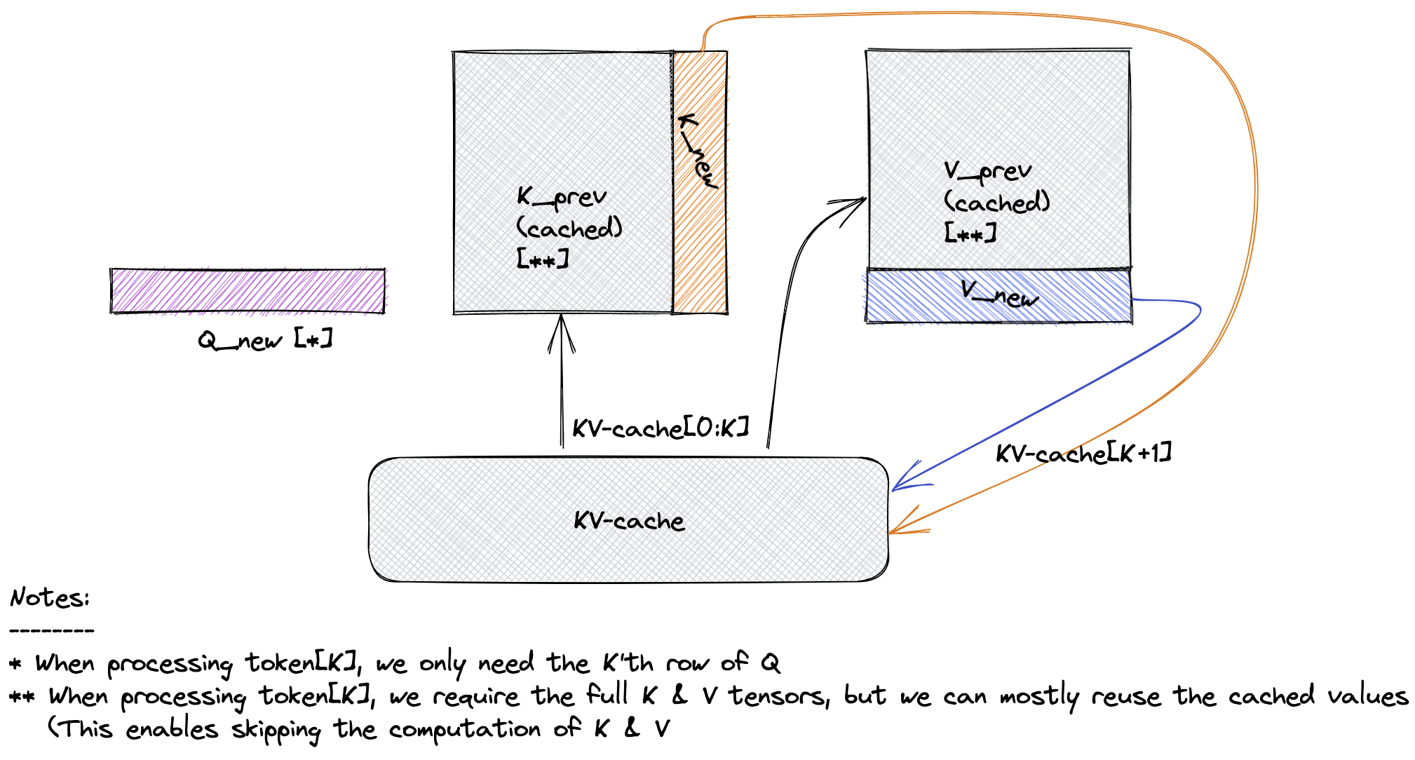
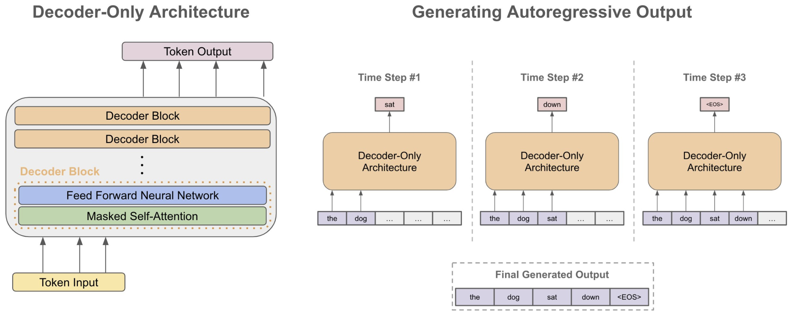
KV-caching is a crucial optimization technique employed in this implementation to accelerate the inference process for Language Model (LM) decoding. During autoregressive decoding, where each token is predicted based on prior tokens, self-attention within the model is causal. This implies that a token's representation is computed based only on itself and the prior tokens, not the future ones.
In self-attention, the input sequence is projected using key, value, and query projections. The KV-cache efficiently stores the results of the key and value projections, eliminating the need for redundant computations in future decoding iterations. As a result, the representations of tokens that remain fixed during autoregressive decoding can be retrieved from the cache, significantly enhancing the inference speed.
This KV-caching technique is a key architectural feature that enhances the efficiency and speed of the LLaMA model during decoding.
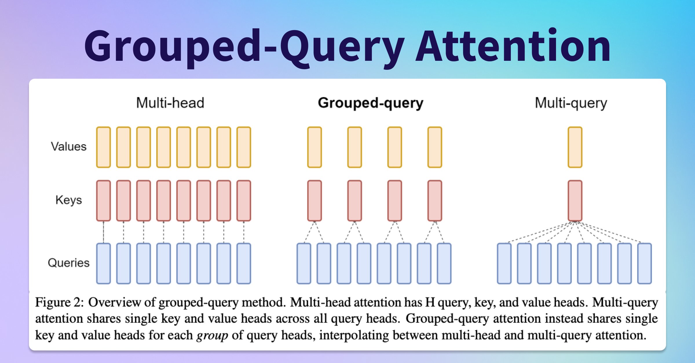
The LLaMA 2 model incorporates a variation of the concept of Multi-Query Attention (MQA) proposed by Shazeer (2019), a refinement of the Multi-Head Attention (MHA) algorithm. MQA enhances the efficiency of attention mechanisms while maintaining minimal accuracy degradation.
In traditional multi-head attention, the entire attention computation is replicated h times, where h is the number of attention heads. However, GQA reduces computational redundancy by removing or significantly reducing the heads dimension (h) from the K and V values. In MQA, each "head" of the query value (Q) undergoes the same K and V transformation, optimizing the attention computation.
This refinement results in similar computational performance to MHA but significantly reduces the amount of data read/written from memory. As a consequence, GQA improves both performance (via an increase in arithmetic intensity) and memory space efficiency (via a decrease in the amount of KV-cache data stored), making it a valuable addition to the LLaMA architecture.
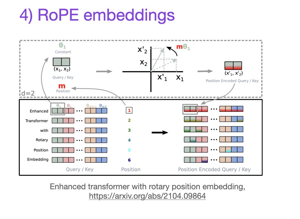
In the LLaMA 2 model, Rotary Positional Embeddings (RoPE) play a crucial role in enhancing attention mechanisms by incorporating positional information into the token representations. The concept of "attention" is powerful, but to ensure that the attention calculated is meaningful, tokens need to have a notion of position.
Position embeddings come in two main types: absolute and relative. Absolute position embeddings encode the absolute position of a word in the input phrase, while relative position embeddings encode the relative position between two words. These embeddings provide vital positional information that helps tokens understand their context in a sequence.
Rotary Positional Embeddings take a unique approach by leveraging rotation matrices to embed positional information. The goal is to ensure that the inner product of vectors q and k, at positions m and n, depends only on q, k, and their relative distance (m — n). The rotation matrix, where the angle is the vector’s position, is embedded into the original vector through matrix multiplication, aligning with this criterion.
This innovative approach to incorporating positional information enhances the model's ability to understand token relationships and context, contributing to improved attention mechanisms.
The model learn a latent representation of the language in a self-supervised way with a surprisingly simple approach: given a large corpus, sequences of fixed size are sampled randomly to build the batched context as input of the model, and the targets are those very same sequences shifted by one element so that the model learn to predict the next token, given a context, by minimizing the cross-entropy through gradient descent:
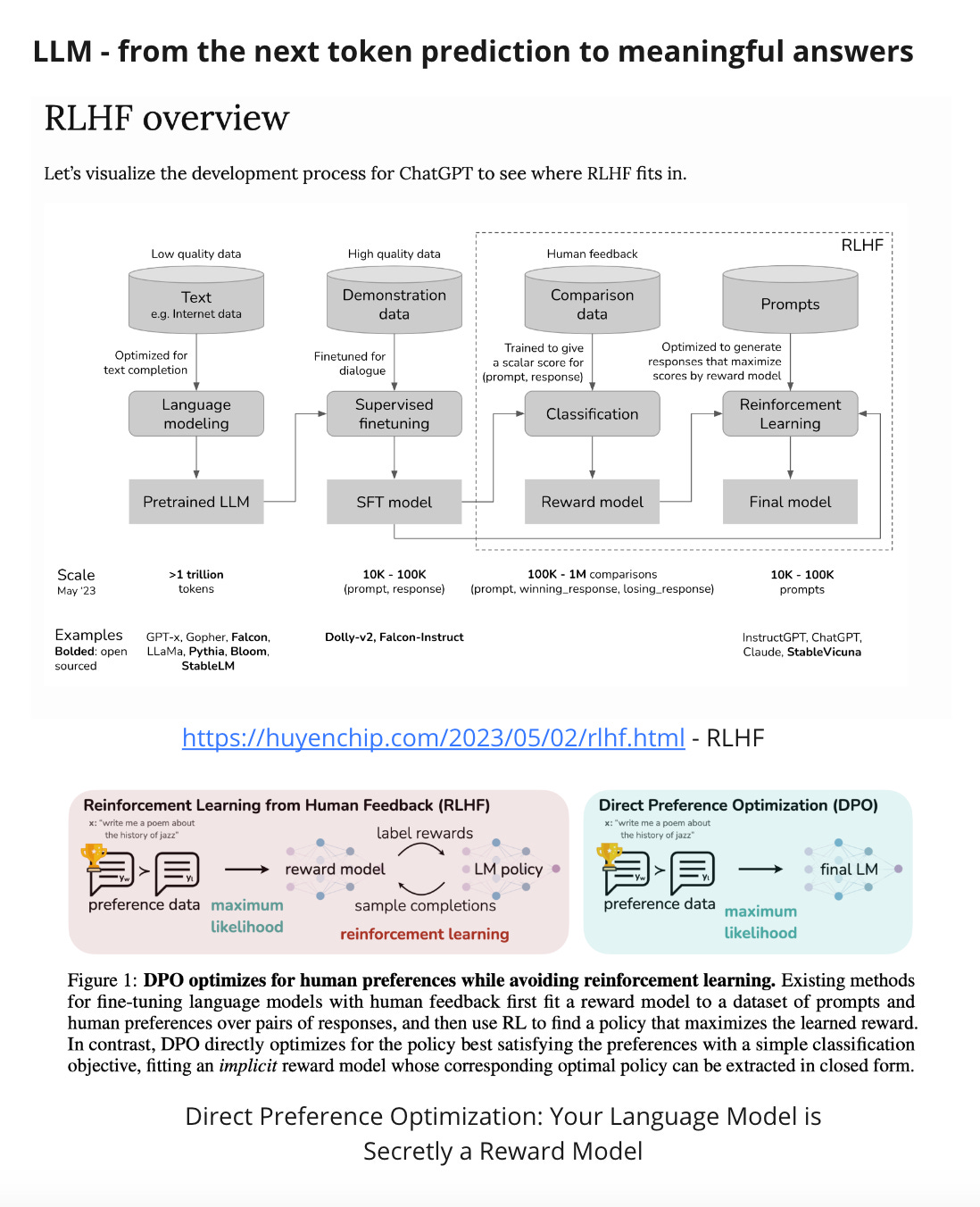
RLHF or reinforcement learning from human feedback is a machine learning technique used to optimize the performance of an AI model through integration of human insight and reinforcement learning. RLHF is highly instrumental in training and fine-tuning GenAI models, including large language models (LLMs), to perform a host of tasks, such as realistic content generation, responding to questions, and code generation. LLMs trained through RLHF generate outputs that are informative and in alignment with human values
- Pre-training: This initial step involves training a model, such as Transformers or Mamba architecture, to predict the next token. While this model can complete sentences, it lacks knowledge of when to stop generating text. Mistral-7B-v0.1 exemplifies a pre-trained model, with over 90% of training dedicated to this step.
import sys

sys.path.append("..")

from pathlib import Path
import matplotlib.pyplot as plt
import torch

from model.llm import LLM
from model.tokenizer import Tokenizer, train_tokenizer

from helpers.dataset import NextTokenPredictionDataset
from helpers.trainer import train
from helpers.config import LLMConfig, TrainingConfig, get_device


print(f"pytorch version: {torch.__version__}")

model = LLM(
    vocab_size=tokenizer.vocab_size,
    context_size=llm_config.context_size,
    dim_emb=llm_config.dim_emb,
    num_layers=llm_config.num_layers,
    attn_num_heads=llm_config.num_heads,
    emb_dropout=llm_config.emb_dropout,
    ffd_hidden_dim=llm_config.ffd_dim_hidden,
    ffd_bias=llm_config.ffd_bias,
)

params_size = sum(p.nelement() * p.element_size() for p in model.parameters())
buffer_size = sum(p.nelement() * p.element_size() for p in model.buffers())
size = (params_size + buffer_size) / 1024**2

print(f"total params: {sum(p.numel() for p in model.parameters()):,d}")
print(f"model size: {size:.3f}MB")

# print(model)-
Supervised Fine-Tuning (SFT): In SFT, the model is trained on high-quality pairs of data, typically request-response pairs. This phase aims to teach the model how to generate answers and when to stop. Although the training objective remains predicting the next token, the data quality improves to reflect real-world usage.
-
Reinforcement Learning from Human Feedback (RLHF): RLHF is pivotal in refining LLMs to generate answers that align with human preferences. Experts compare different model-generated answers to a question and provide feedback. This feedback is used to train a reward model, which guides further optimization of the LLM after SFT.
import torch.nn as nn
import torch

class PPOTrainer:
    def __init__(
        self,
        args,
        tokenizer: PreTrainedTokenizer,
        policy_model: PreTrainedModel,
        value_model: nn.Module,
        reward_model: Callable,
        optimizer: torch.optim.Optimizer,
    ) -> None:
        self.config = args
        self.tokenizer = tokenizer
        self.policy_model = policy_model
        self.value_model = value_model
        self.reward_model = reward_model
        self.optimizer = optimizer

    def compute_advantages(
        self,
        values: torch.Tensor,
        rewards: torch.Tensor,
        mask: torch.Tensor,
    ) -> tuple[torch.Tensor, torch.Tensor, torch.Tensor]:
        lastgaelam = 0
        advantages_reversed = []
        gen_len = rewards.shape[-1]

        values = values * mask
        rewards = rewards * mask

        for t in reversed(range(gen_len)):
            nextvalues = values[:, t + 1] if t < gen_len - 1 else 0.0
            delta = rewards[:, t] + self.config.gamma * nextvalues - values[:, t]
            lastgaelam = delta + self.config.gamma * self.config.lam * lastgaelam
            advantages_reversed.append(lastgaelam)
        advantages = torch.stack(advantages_reversed[::-1]).transpose(0, 1)

        returns = advantages + values
        advantages = masked_whiten(advantages, mask)
        advantages = advantages.detach()
        return values, advantages, returns

    @torch.no_grad()
    def sample_experience(self, prompt_ids: torch.Tensor, prompt_mask: torch.Tensor) -> dict[str, torch.Tensor]:
        self.policy_model.eval()
        self.value_model.eval()

        _, prompt_length = prompt_ids.shape

        input_ids = self.policy_model.generate(
            input_ids=prompt_ids,
            attention_mask=prompt_mask,
            max_length=self.config.max_length,
            use_cache=True,
            do_sample=self.config.temp > 0,
            temperature=self.config.temp,
            top_p=self.config.top_p,
            eos_token_id=[self.tokenizer.eos_token_id, self.tokenizer.pad_token_id],
            pad_token_id=self.tokenizer.pad_token_id,
        )

        attention_mask = (input_ids != self.tokenizer.pad_token_id).long()
        old_logits = self.policy_model(input_ids, attention_mask=attention_mask).logits
        rewards = self.reward_model(input_ids=input_ids, attention_mask=attention_mask)
        values = self.value_model(input_ids=input_ids, attention_mask=attention_mask)

        old_logprobs = logprobs_from_logits(old_logits[:, :-1, :], input_ids[:, 1:])

        mask = attention_mask[:, prompt_length:]
        rewards = rewards[:, prompt_length:]
        values = values[:, prompt_length - 1 : -1]
        old_logprobs = old_logprobs[:, prompt_length - 1 :]

        values, advantages, returns = self.compute_advantages(values, rewards, mask)

        return dict(
            prompt_ids=prompt_ids,
            old_logprobs=old_logprobs,
            values=values,
            rewards=rewards,
            input_ids=input_ids,
            attention_mask=attention_mask,
            advantages=advantages,
            returns=returns,
        )

    def train_minibatch(self, inputs: dict[str, torch.Tensor]) -> dict[str, torch.Tensor]:
        self.policy_model.train()
        self.value_model.train()

        prompt_ids = inputs["prompt_ids"]
        old_logprobs = inputs["old_logprobs"]
        rewards = inputs["rewards"]
        values = inputs["values"]
        attention_mask = inputs["attention_mask"]
        input_ids = inputs["input_ids"]
        advantages = inputs["advantages"]
        returns = inputs["returns"]

        _, prompt_length = prompt_ids.shape
        mask = attention_mask[:, prompt_length:]

        logits = self.policy_model(input_ids=input_ids, attention_mask=attention_mask, use_cache=False).logits
        logprobs = logprobs_from_logits(logits[:, :-1, :], input_ids[:, 1:])
        logprobs = logprobs[:, prompt_length - 1 :]

        entropy = masked_mean(entropy_from_logits(logits[:, prompt_length - 1 : -1]), mask)
        approxkl = 0.5 * masked_mean((logprobs - old_logprobs) ** 2, mask)
        policykl = masked_mean(old_logprobs - logprobs, mask)

        ratio = torch.exp(logprobs - old_logprobs)
        pg_losses1 = -advantages * ratio
        pg_losses2 = -advantages * torch.clamp(ratio, 1.0 - self.config.cliprange, 1.0 + self.config.cliprange)
        pg_loss = masked_mean(torch.max(pg_losses1, pg_losses2), mask)
        pg_clipfrac = masked_mean((pg_losses2 > pg_losses1).float(), mask)

        vpreds = self.value_model(input_ids=input_ids, attention_mask=attention_mask)
        vpreds = vpreds[:, prompt_length - 1 : -1]

        vpredclipped = torch.clamp(
            vpreds, min=values - self.config.cliprange_value, max=values + self.config.cliprange_value
        )
        vf_losses1 = (vpreds - returns) ** 2
        vf_losses2 = (vpredclipped - returns) ** 2
        vf_loss = 0.5 * masked_mean(torch.max(vf_losses1, vf_losses2), mask)
        vf_clipfrac = masked_mean((vf_losses2 > vf_losses1).float(), mask)

        loss = pg_loss + self.config.vf_coef * vf_loss

        loss.backward()
        pg_grad_norm = nn.utils.clip_grad_norm_(self.policy_model.parameters(), max_norm=self.config.max_grad_norm)
        vf_grad_norm = nn.utils.clip_grad_norm_(
            self.value_model.parameters(), max_norm=self.config.max_grad_norm * self.config.vf_coef
        )
        self.optimizer.step()
        self.optimizer.zero_grad()

        stats = {
            **{f"lr/group_{i}": pg["lr"] for i, pg in enumerate(self.optimizer.param_groups)},
            "loss/policy": pg_loss.item(),
            "loss/value": vf_loss.item(),
            "loss/total": loss.item(),
            "policy/grad_norm": pg_grad_norm.item(),
            "policy/entropy": entropy.item(),
            "policy/approxkl": approxkl.item(),
            "policy/policykl": policykl.item(),
            "policy/clipfrac": pg_clipfrac.item(),
            "policy/advantages_mean": masked_mean(advantages, mask).item(),
            "policy/advantages_var": masked_var(advantages, mask).item(),
            "policy/ratio_mean": masked_mean(ratio, mask).item(),
            "returns/mean": masked_mean(returns, mask).item(),
            "returns/var": masked_var(returns, mask).item(),
            "val/grad_norm": vf_grad_norm.item(),
            "val/vpred": masked_mean(vpreds, mask).item(),
            "val/error": masked_mean(vf_losses1, mask).item(),
            "val/clipfrac": vf_clipfrac.item(),
            "val/mean": masked_mean(values, mask).item(),
            "val/var": masked_var(values, mask).item(),
            "env/reward_mean": masked_mean(rewards, mask).item(),
            "env/reward_var": masked_var(rewards, mask).item(),
            "env/reward_total": rewards.sum(1).mean().item(),
        }
        return stats


class GoldenRewardModel:
    def __init__(self, tokenizer: PreTrainedTokenizer) -> None:
        self.tokenizer = tokenizer

    def __call__(self, input_ids: torch.Tensor, attention_mask: torch.Tensor, **kwargs) -> torch.Tensor:
        batch_size, seq_len = input_ids.shape
        input_ids_list = input_ids.tolist()
        prompt_length = input_ids_list[0].index(self.tokenizer.eos_token_id) + 1

        scores = [[0 for _ in range(seq_len)] for _ in range(batch_size)]
        for input_id, score in zip(input_ids_list, scores):
            prompt_id = input_id[:prompt_length]
            target_id = [x for x in prompt_id if x != self.tokenizer.pad_token_id]
            response_id = input_id[prompt_length:]
            for j, (rsp_id, tgt_id) in enumerate(zip(response_id, target_id)):
                if rsp_id != tgt_id:
                    break
                score[prompt_length + j] = 1

return torch.tensor(scores, dtype=torch.float32, device=input_ids.device)We have learned a lot from the open source community and we appreciate the below projects:
- huggingface/trl: most of our PPO implementation is adapted from trl.
- DeepSpeed-Chat: the training pipeline are adapted from DS-Chat, then made even simpler


