Liang Yu: yuliang@mit.edu
This directory contains TensorFlow models and data processing code for identifying exoplanets in astrophysical light curves. For complete background on how CNNs work for planet detection, see Shallue & Vanderburg's paper in The Astronomical Journal. This is the vetting version of our two TESS neural networks. For the triage version, see https://github.com/yuliang419/Astronet-Triage.
For shorter summaries, see:
- "Earth to Exoplanet" on the Google blog
- This blog post by Andrew Vanderburg
- This great article by Fedor Kossakovski
- NASA's press release article
A paper that summarizes this code is available here and at The Astronomical Journal. Please cite it if you make use of this code:
Yu, L. et al. (2019). Identifying Exoplanets with Deep Learning III: Automated Triage and Vetting of TESS Candidates. The Astronomical Journal, 158(1), 25.
See also the original Shallue & Vanderburg paper:
Shallue, C. J., & Vanderburg, A. (2018). Identifying Exoplanets with Deep Learning: A Five-planet Resonant Chain around Kepler-80 and an Eighth Planet around Kepler-90. The Astronomical Journal, 155(2), 94.
Full text available at The Astronomical Journal.
- TensorFlow code for:
- Downloading and preprocessing TESS data.
- Building different types of neural network classification models.
- Training and evaluating a new model.
- Using a trained model to generate new predictions.
- Utilities for operating on light curves. These include:
- Reading TESS data from
.h5files. - Phase folding, splitting, binning, etc.
- Reading TESS data from
- In addition, some C++ implementations of light curve utilities are located in light_curve_util/cc/.
- Utilities derived from third party code.
First, ensure that you have installed the following required packages:
- TensorFlow (instructions)
- Pandas (instructions)
- NumPy (instructions)
- AstroPy (instructions)
- PyDl (instructions)
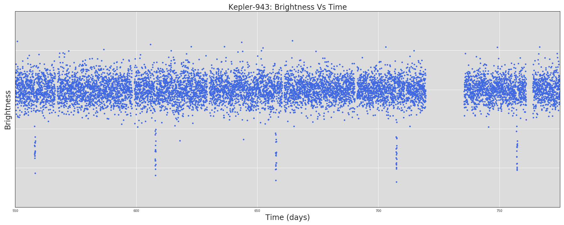
A light curve is a plot of the brightness of a star over time. We will be focusing on light curves produced by the TESS space telescope. An example light curve (produced by Kepler) is shown below.
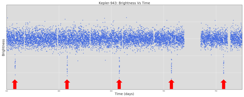
To train a model to identify planets in TESS light curves, you will need a training set of labeled Threshold Crossing Events (TCEs). A TCE is a periodic signal that has been detected in a Kepler light curve, and is associated with a period (the number of days between each occurrence of the detected signal), a duration (the time taken by each occurrence of the signal), an epoch (the time of the first observed occurrence of the signal), and possibly additional metadata like the signal-to-noise ratio. An example TCE is shown below. The labels are ground truth classifications (decided by humans) that indicate which TCEs in the training set are actual planets signals and which are caused by other phenomena.
The CSV creation step needs to be run on PDO, but I have included the complete CSV file (astronet/tces.csv) that I used to train the model.
The TESS TCE lists for each sector are available on the TEV website. Download them as CSVs, and run make_catalog.py in the data folder to create a catalog that combines all sectors. e.g.:
python make_catalog.py --input sector-1-earlylook.csv sector-2-bright.csv sector-3-01.csv sector-3-02.csv --num_worker_processes=20 --base_dir=[wherever your csv file is] --out_name=tces.csv
The output will be a CSV file named tces.csv (in the same directory as your input CSV file) with the following columns:
row_id: Integer ID of the row in the TCE table.tic_id: TIC ID of the target star.toi_id: TCE number within the target star. These are structured funny so we'll ignore them for now.Disposition: Final disposition from group vetting (should be one of the following: PC (planet candidate), EB (eclipsing binary), IS (instrumental noise), V (variability), O (other), J (junk). The J class includes a mix of V and IS. I didn't distinguish all of them since these two are always lumped together anyway.RA: RA in degrees.DEC: Dec in degrees.Tmag: TESS magnitude.Epoc: The time corresponding to the center of the first detected event in Barycentric Julian Day (BJD) minus a constant offset.Period: Period of the detected event, in days.Duration: Duration of the detected event, in hours.Transit Depth: Transit depth in ppm.Sectors: Sector number.camera: Camera number.ccd: CCD number.star_rad,star_mass,teff,logg: Stellar parameters from Gaia DR2 or the TIC. Since a lot of TCEs are missing these values, we're not using them right now.SN: Signal-to-pink noise ratio from BLS.q_ingress: Fractional ingress duration from VARTOOLS.
The catalog creation step may take a while to run, depending on how many TCEs there are. For entire sectors, I'd recommend using at least 20 workers in parallel, or it will take forever. Set num_worker_processes to 1 to turn off multiprocessing.
Light curves are stored as h5 files on PDO, in e.g. /pdo/qlp-data/sector-2/ffi/cam1/ccd1/LC/ . Download all the light curves you need from one sector and store them in a local directory called astronet/tess/sector-X (no need to subdivide by camera and ccd).
If working with TCEs that are not available on TEV, start by creating a .txt file of TIC IDs of all TCEs that you wish to include, and name the file sector-x-yyy.txt, where x is the sector number and yyy is an optional string. Then run make_empty_catalog.py in the data directory to create a csv file in a specified location (named sector-X-all.csv) with only a few columns filled in, e.g.:
python make_empty_catalog.py --base_dir=[wherever you text file is] --input sector-4-bad.txt sector-4-good.txt --save_dir=[wherever you want to save the output]
Note that the csv file created this way will have a disposition of J for all TCEs, because I mostly used this to create catalogs of junk that didn't make it to group vetting.
Then, run make_catalog.py as usual to create a CSV file with the rest of the columns filled in.
All the following steps can be run on any computer that has TESS h5 files stored in a single folder, divided by sector. If you don't have access to the original h5 files, I have included all the TFRecords used in my paper under astronet/tfrecords so you can skip the training set generation step.
To train a model to identify exoplanets, you will need to provide TensorFlow
with training data in
TFRecord format. The
TFRecord format consists of a set of sharded files containing serialized
tf.Example protocol buffers.
The command below will generate a set of sharded TFRecord files for the TCEs in
the training set. Each tf.Example proto will contain the following light curve
representations:
global_view: Vector of length 201: a "global view" of the TCE.local_view: Vector of length 61: a "local view" of the TCE.
In addition, each tf.Example will contain the value of each column in the
input TCE CSV file, including transit and stellar parameters.
Disclaimer: I haven't figured out how to make Bazel work, so just use the plain python version for now.
To generate the training set:
# The original Astronet used Bazel, but we could just invoke the source scripts with the
# following addition to PYTHONPATH:
export PYTHONPATH="/path/to/source/dir/:${PYTHONPATH}"

# Filename containing the CSV file of TCEs in the training set.
TCE_CSV_FILE="astronet/tces.csv"

# Directory to save output TFRecord files into.
TFRECORD_DIR="astronet/tfrecord"

# Directory where light curves are located.
TESS_DATA_DIR="astronet/tess/"

# Run without bazel
python astronet/data/generate_input_records.py \
--input_tce_csv_file=${TCE_CSV_FILE} \
--tess_data_dir=${TESS_DATA_DIR} \
--output_dir=${TFRECORD_DIR} \
--num_worker_processes=5
If --clean is included as an argument, the train and validation sets will only contain TCEs with S/N above some threshold (specified by the --threshold argument, default 15).
If the optional --make_test_set argument is included, the code will generate 8 test sets instead of 8 training, 1 validation and 1 test. This is useful for creating test sets out of new data and using them to evaluate a model trained on older data. Setting --clean here would produce test sets containing only TCEs with S/N above some threshold.
When the script finishes you will find 8 training files, 1 validation file and
1 test file in TFRECORD_DIR. The files will match the patterns
train-0000?-of-00008, val-00000-of-00001 and test-00000-of-00001
respectively.
Here's a quick description of what the script does. For a full description, see Section 3 of our paper.
For TESS light curves, background variability has already been removed (mostly), so the spline-fitting step in the original paper is not necessary.
For each TCE in the input CSV table, we generate two representations of the light curve of that star. Both representations are phase-folded, which means that we combine all periods of the detected TCE into a single curve, with the detected event centered.
Here's an example of the generated representations (Kepler-90 g) in the output.
# Launch iPython (or Python) from the tensorflow_models/astronet/ directory.
ipython

In[1]:
import matplotlib.pyplot as plt
import numpy as np
import os.path
import tensorflow as tf

In[2]:
TIC_ID = 270341214
TFRECORD_DIR = "/path/to/tfrecords/dir"

In[3]:
# Helper function to find the tf.Example corresponding to a particular TCE.
def find_tce(tic_id, filenames):
  for filename in filenames:
    for record in tf.python_io.tf_record_iterator(filename):
      ex = tf.train.Example.FromString(record)
      if ex.features.feature["tic_id"].int64_list.value[0] == tic_id:
        print("Found {} in file {}".format(tic_id, filename))
        return ex
        raise ValueError("{} not found in files: {}".format(tic_id, filenames))

In[4]:
# Find sample TCE
filenames = tf.gfile.Glob(os.path.join(TFRECORD_DIR, "*"))
assert filenames, "No files found in {}".format(TFRECORD_DIR)
ex = find_tce(TIC_ID, filenames)

In[5]:
# Plot the global and local views.
global_view = np.array(ex.features.feature["global_view"].float_list.value)
local_view = np.array(ex.features.feature["local_view"].float_list.value)
fig, axes = plt.subplots(1, 2, figsize=(20, 6))
axes[0].plot(global_view, ".")
axes[1].plot(local_view, ".")
plt.show()
The output should look something like this:
The astronet directory contains several types of neural network architecture and various configuration options. This particular version is configured to detect objects that can plausibly be planets (including PCs and EBs whose stellar variability amplitudes are less than half the depths of the eclipses). To train a convolutional neural network to classify TESS TCEs as either "likely planet" or "not planet", using the best configuration from our paper, run the following training script:
# Directory to save model checkpoints into.
MODEL_DIR="astronet/model/"

# Run without Bazel
python astronet/train.py \
--model=AstroCNNModel \
--config_name=local_global \
--train_files=${TFRECORD_DIR}/train* \
--eval_files=${TFRECORD_DIR}/val* \
--model_dir=${MODEL_DIR} \
--train_steps=14000
Optionally, you can also run a TensorBoard server in a separate process for real-time monitoring of training progress and evaluation metrics.
# Launch TensorBoard server.
tensorboard --logdir ${MODEL_DIR}
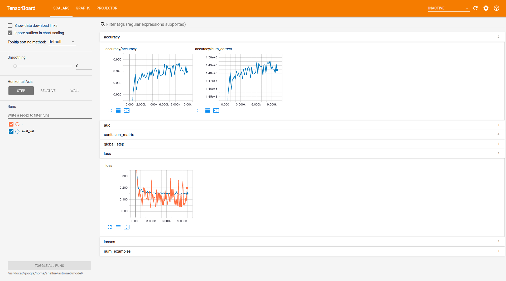
The TensorBoard server will show a page like this:
The "loss" plot shows both training and validation losses. The optimum number of training steps is where validation loss reaches a minimum.
You can train a set of 10 models with random initializations and average their outputs when making predictions. This helps prevent overfitting and makes the model more robust. To do this, use the following command:
./astronet/ensemble_train.sh ${MODEL_DIR} 14000 ${TFRECORD_DIR}The 14000 here is the number of train steps I used for each model. The code will produce 10 subdirectories under ${MODEL_DIR}.
Four fully trained, averaged models can be found under astronet/models_final. model_dc_se is the final version presented in my paper, with secondary eclipses and depth change included in the model. model_plain is the original AstroNet architecture without the two newly added features. model_dc and model_se are models with only depth change or only secondary eclipses added.
Run the following command to evaluate a model on the test set. The result will be printed on the screen, and a summary file will also be written to the model directory, which will be visible in TensorBoard.
# Run evaluation script
python astronet/evaluate.py \
--model=AstroCNNModel \
--config_name=local_global \
--eval_files=${TFRECORD_DIR}/test* \
--model_dir=${MODEL_DIR}
The output should look something like this:
INFO:tensorflow:Saving dict for global step 10000: accuracy/accuracy = 0.9625159, accuracy/num_correct = 1515.0, auc = 0.988882, confusion_matrix/false_negatives = 10.0, confusion_matrix/false_positives = 49.0, confusion_matrix/true_negatives = 1165.0, confusion_matrix/true_positives = 350.0, global_step = 10000, loss = 0.112445444, losses/weighted_cross_entropy = 0.11295206, num_examples = 1574.To plot the misclassified TCEs and calculate precision and recall at various thresholds, do the following:
python astronet/find_incorrect.py --model_dir=${MODEL_DIR} --tfrecord_dir=${TFRECORD_DIR} --suffix=yyy --averageThis produces plots of the global and local views of misclassified TCEs in a folder called astronet/plots and generates a text file called true_vs_pred_yyy.txt with two columns: the true disposition of each TCEs in the test set (0 = junk, 1 = PC or EB), the predicted probability of each TCE being a positive. If you trained an ensemble of models and want to use model averaging, include a --average argument and make sure ${MODEL_DIR} is set to the directory that contains the 10 subdirectories. If there's no --average argument, ${MODEL_DIR} is just the directory containing your single model.
To plot the precision-recall curve, run plot_roc.py with the appropriate true_vs_pred file (you'll have to modify the code directly).
The easiest way to make predictions for a list of new TCEs is to run generate_input_records.py following instructions above with the --make_test_set argument included, such that all the new TCEs to be classified are stored as tfrecords. Then run the following:
# Make a directory for plots
mkdir astronet/plots
SAVE_DIR=astronet/plots

# Generate a prediction for a list of new TCEs.
python astronet/batch_predict.py \
  --model_dir=${MODEL_DIR} \
  --tfrecord_dir=${TFRECORD_DIR} \
  --suffix=yyy \
  --average \
  --plot \
  --save_dir=${SAVE_DIR}
If the option --plot argument is included, you must also include a --save_dir. Plots of the global and local views of TCEs in the test set will be saved under that directory.
If you trained an ensemble of models and want to use model averaging, include a --average argument and make sure ${MODEL_DIR} is set to the directory that contains the 10 subdirectories. If there's no --average argument, ${MODEL_DIR} is just the directory containing your single model.
The output of this step is a file called prediction_yyy.txt, saved in your current directory. This file contains the TIC ID of each object in your input list, and the model's prediction of the object being a plausible planet candidate. In this version (triage), that means the object is likely either a PC or an EB without too much stellar activity.


