Bayesian Generative Adversarial Networks in Tensorflow

This repository contains the Tensorflow implementation of the Bayesian GAN by Yunus Saatchi and Andrew Gordon Wilson. This paper will be appearing at NIPS 2017.

The bibliographic information for the paper is

@inproceedings{saatchiwilson2017,
  title={Bayesian {GAN}},
  author={Saatchi, Yunus and Wilson, Andrew Gordon},
  booktitle={Advances in Neural Information Processing Systems},
  year={2017}
}

Introduction
Dependencies
Training options
Usage

Introduction

In the Bayesian GAN we propose conditional posteriors for the generator and discriminator weights, and marginalize these posteriors through stochastic gradient Hamiltonian Monte Carlo. Key properties of the Bayesian approach to GANs include (1) accurate predictions on semi-supervised learning problems; (2) minimal intervention for good performance; (3) a probabilistic formulation for inference in response to adversarial feedback; (4) avoidance of mode collapse; and (5) a representation of multiple complementary generative and discriminative models for data, forming a probabilistic ensemble.

We illustrate a multimodal posterior over the parameters of the generator. Each setting of these parameters corresponds to a different generative hypothesis for the data. We show here samples generated for two different settings of this weight vector, corresponding to different writing styles. The Bayesian GAN retains this whole distribution over parameters. By contrast, a standard GAN represents this whole distribution with a point estimate (analogous to a single maximum likelihood solution), missing potentially compelling explanations for the data.

Dependencies

This code has the following dependencies (version number crucial):

python 2.7
tensorflow==1.0.0

To install tensorflow 1.0.0 on linux please follow instructions at https://www.tensorflow.org/versions/r1.0/install/.

scikit-learn==0.17.1

You can install scikit-learn 0.17.1 with the following command

pip install scikit-learn==0.17.1

Alternatively, you can create a conda environment and set it up using the provided environment.yml file, as such:

conda env create -f environment.yml -n bgan

then load the environment using

source activate bgan

Training options

bayesian_gan_hmc.py has the following training options.

--out_dir: path to the folder, where the outputs will be stored
--n_save: samples and weights are saved every n_save iterations; default 100
--z_dim: dimensionalit of z vector for generator; default 100
--data_path: path to the data; see data preparation for a detailed discussion; this parameter is required
--dataset: can be mnist, cifar, svhn or celeb; default mnist
--gen_observed: number of data "observed" by the generator; this affects the scaling of the noise variance and prior; default 1000
--batch_size: batch size for training; default 64
--prior_std: std of the prior distribution over the weights; default 1
--numz: same as J in the paper; number of samples of z to integrate it out; default 1
--num_mcmc: same as M in the paper; number of MCMC NN weight samples per z; default 1
--lr: learning rate used by the Adam optimizer; default 0.0002
--optimizer: optimization method to be used: adam (tf.train.AdamOptimizer) or sgd (tf.train.MomentumOptimizer); default adam
--semi_supervised: do semi-supervised learning
--N: number of labeled samples for semi-supervised learning
--train_iter: number of training iterations; default 50000
--save_samples: save generated samples during training
--save_weights: save weights during training
--random_seed: random seed; note that setting this seed does not lead to 100% reproducible results if GPU is used

You can also run WGANs with --wasserstein or train an ensemble of <num_dcgans> DCGANs with --ml_ensemble <num_dcgans>. In particular you can train a DCGAN with --ml_ensemble 1.

Usage

Installation

Install the required dependencies
Clone this repository

Synthetic Data

To run the synthetic experiment from the paper you can use bgan_synth script. For example, the following comand will train the Bayesian GAN (with D=100 and d=10) for 5000 iterations and store the results in <results_path>.

./bgan_synth.py --x_dim 100 --z_dim 10 --numz 10 --out <results_path>

To run the ML GAN for the same data run

./bgan_synth.py --x_dim 100 --z_dim 10 --numz 1 --out <results_path>

bgan_synth has --save_weights, --out_dir, --z_dim, --numz, --wasserstein, --train_iter and --x_dim parameters. x_dim contolls the dimensionality of the observed data (x in the paper). For description of other parameters please see Training options.

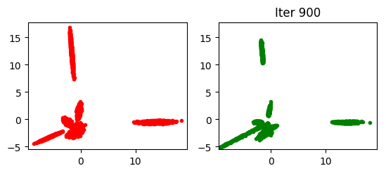
Once you run the above two commands you will see the output of each 100th iteration in <results_path>. So, for example, the Bayesian GAN's output at the 900th iteration will look like:

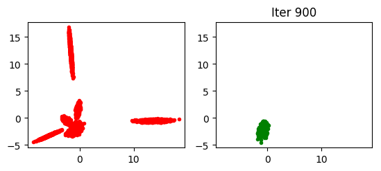
In contrast, the output of the standard GAN (corresponding to numz=1, which forces ML estimation) will look like:

indicating clearly the tendency of mode collapse in the standard GAN which, for this synthetic example, is completely avoided by the Bayesian GAN.

To explore the sythetic experiment further, and to generate the Jensen-Shannon divergence plots, you can check out the notebook synth.ipynb.

MNIST, CIFAR10, CelebA, SVHN

bayesian_gan_hmc script allows to train the model on standard and custom datasets. Below we describe the usage of this script.

Data preparation

To reproduce the experiments on MNIST, CIFAR10, CelebA and SVHN datasets you need to prepare the data and use a correct --data_path.

for MNIST you don't need to prepare the data and can provide any --data_path;
for CIFAR10 please download and extract the python version of the data from https://www.cs.toronto.edu/~kriz/cifar.html; then use the path to the directory containing cifar-10-batches-py as --data_path;
for SVHN please download train_32x32.mat and test_32x32.mat files from http://ufldl.stanford.edu/housenumbers/ and use the directory containing these files as your --data_path;
for CelebA you will need to have openCV installed. You can find the download links for the data at http://mmlab.ie.cuhk.edu.hk/projects/CelebA.html. You will need to create celebA folder with Anno and img_align_celeba subfolders. Anno must contain the list_attr_celeba.txt and img_align_celeba must contain the .jpg files. You will also need to crop the images by running datasets/crop_faces.py script with --data_path <path> where <path> is the path to the folder containing celebA. When training the model, you will need to use the same <path> for --data_path;

Unsupervised training

You can train the model in unsupervised way by running the bayesian_gan_hmc script without --semi parameter. For example, use

./bayesian_gan_hmc.py --data_path <data_path> --dataset svhn --numz 1 --num_mcmc 10 --out_dir 
<results_path> --train_iter 75000 --save_samples --n_save 100

to train the model on the SVHN dataset. This command will run the method for 75000 iterations and save samples every 100 iterations. Here <results_path> must lead to the directory where the results will be stored. See data preparation section for an explanation of how to set <data_path>. See training options section for a description of other training options.

Semi-supervised training

You can train the model in semi-supervised setting by running bayesian_gan_hmc with --semi option. Use -N parameter to set the number of labeled examples to train on. For example, use

./bayesian_gan_hmc.py --data_path <data_path> --dataset cifar --numz 1 --num_mcmc 10
--out_dir <results_path> --train_iter 75000 --N 4000 --semi --lr 0.00005

to train the model on CIFAR10 dataset with 4000 labeled examples. This command will train the model for 75000 iterations and store the outputs in <results_path> folder.

To train the model on MNIST with 200 labeled examples you can use the following command.

./bayesian_gan_hmc.py --data_path <data_path>/ --dataset mnist --numz 5 --num_mcmc 5
--out_dir <results_path> --train_iter 30000 -N 200 --semi --lr 0.001

Custom data

To train the model on a custom dataset you need to define a class with a specific interface. Suppose we want to train the model on the digits dataset. This datasets consists of 8x8 images of digits. Let's suppose that the data is stored in x_tr.npy, y_tr.npy, x_te.npy and y_te.npy files. We will assume that x_tr.npy and x_te.npy have shapes of the form (?, 8, 8, 1). We can then define the class corresponding to this dataset in bgan_util.py as follows.

class Digits:

    def __init__(self):
        self.imgs = np.load('x_tr.npy') 
        self.test_imgs = np.load('x_te.npy')
        self.labels = np.load('y_tr.npy')
        self.test_labels = np.load('y_te.npy')
        self.labels = one_hot_encoded(self.labels, 10)
        self.test_labels = one_hot_encoded(self.test_labels, 10) 
        self.x_dim = [8, 8, 1]
        self.num_classes = 10

    @staticmethod
    def get_batch(batch_size, x, y): 
        """Returns a batch from the given arrays.
        """
        idx = np.random.choice(range(x.shape[0]), size=(batch_size,), replace=False)
        return x[idx], y[idx]

    def next_batch(self, batch_size, class_id=None):
        return self.get_batch(batch_size, self.imgs, self.labels)

    def test_batch(self, batch_size):
        return self.get_batch(batch_size, self.test_imgs, self.test_labels)

The class must have next_batch and test_batch, and must have the imgs, labels, test_imgs, test_labels, x_dim and num_classes fields.

Now we can import the Digits class in bayesian_gan_hmc.py

from bgan_util import Digits

and add the following lines to to the processing of --dataset parameter.

if args.dataset == "digits":
    dataset = Digits()

After this preparation is done, we can train the model with, for example,

./bayesian_gan_hmc.py --data_path <any_path> --dataset digits --numz 1 --num_mcmc 10 
--out_dir <results path> --train_iter 5000 --save_samples

Acknowledgements

We thank Pavel Izmailov for help with stress testing this code and creating the tutorial.

13331151/bayesgan