Copyright © 2023, Georgia Institute of Technology. All rights reserved.
Machine Learning for AC Optimal Power Flow(ACOPF) benchmark for VNNCOMP
To set up the environment, follow these steps:
- Create the environment using the command:
conda env create -f env.yaml - Activate the environment using the command:
conda activate onnx-vnnlib-env
The benchmark files are located in the onnx and vnnlib folders:
To reproduce vnnlib files, run: python generate_properties.py
+- a% perturbation of the reference active and reactive load + random noise between -b% and b%, where a and b are self-defined values.
Check the properties of the NN output
For example, we are interested in if power balance violation is within some threshold:
for each bus i
|p_balance[i]| <= max(10^(-3), 10^(-2)*pd_i)|q_balance[i]| <= max(10^(-3), 10^(-2)*qd_i)
where pd_i and qd_i refer to the active and reactive load at each bus respectively.
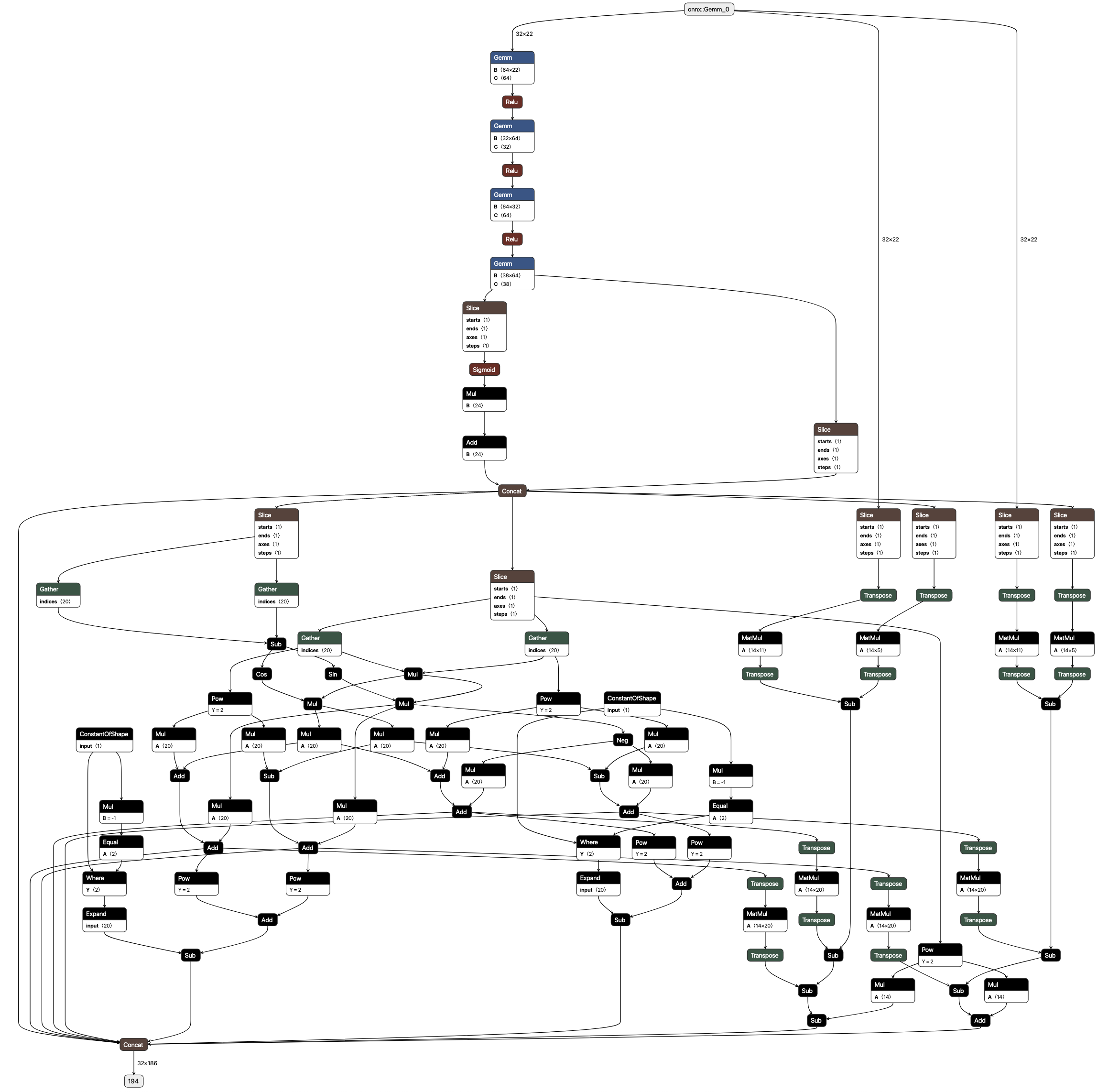
The code to run inference is presented in the main.py file.
Take 14-bus system as an example:
- onnx file:
14_ieee_ml4acopf.onnx - vnnlib file:
14_ieee_prop1.vnnlib
- N = 14 : number of buses
- G = 5 : number of generators
- L = 11 : number of loads
- E = 20 : number of lines
dim: (2L) = 22
pd: Real power demand. (L)qd: Reactive power demand. (L)
dim: (2G + 4N + 6E) = 186
pg: Real power generation. (G)qg: Reactive power generation. (G)vm: Voltage magnitude. (N)va: Voltage angle. (N)pf: Real power flow from. (E)pt: Real power flow to. (E)qf: Reactive power flow from. (E)qt: Reactive power flow to. (E)thrm_1: Thermal limit from residual. (E)thrm_2: Thermal limit to residual. (E)p_balance: Real power balance residual. (N)q_balance: Reactive power balance residual. (N)
