enhanced-srgan

Abstract

Image super-resolution (SR) is the process of recovering high-resolution (HR) images from low-resolution (LR) images. It is an important class of image processing techniques in computer vision and image processing with a wide range of real-world applications, such as medical imaging, satellite imaging, surveillance and security, and astronomical imaging.

With the fast progress in deep learning techniques in recent years, deep learning-based SR models have been actively explored and often achieve state-of-the-art performance on various benchmarks of super-resolution tasks. Several deep learning methods have been applied to solve SR tasks, ranging from the early Convolutional Neural Networks (CNN) based models to recent promising Generative Adversarial network-based SR approaches.

In this project, we implement the Enhanced Super-Resolution Generative Adversarial Network (ESRGAN), capable of generating realistic textures when performing single image super-resolution (SISR). This implementation was introduced by Xintao et al. in 2018 in the paper ESRGAN: Enhanced Super-Resolution Generative Adversarial Networks, based on the original work shown in the paper Photo-Realistic Single Image Super-Resolution Using a Generative Adversarial Network by Ledig et al., from which it implements a series of improvements to the three principal components of the deep learning model: the network architecture, adversarial loss, and perceptual loss.

Authors: Marc Bermejo, Ferran Torres, Raul Puente

1. Introduction

Single image super-resolution (SISR), as a fundamental low-level vision problem, has attracted increasing attention in the research community and AI companies. SISR aims at recovering a high-resolution (HR) image from a single low-resolution (LR) one. Since the pioneer work of SRCNN proposed by Dong et al., deep convolution neural network (CNN) approaches have brought prosperous development. Various network architecture designs and training strategies have continuously improved the SR performance, especially the Peak Signal-to-Noise Ratio (PSNR) value. However, these PSNR-oriented approaches tend to output over-smoothed results without sufficient high-frequency details, since the PSNR metric fundamentally disagrees with the subjective evaluation of human observers.

Several perceptual-driven methods have been proposed to improve the visual quality of SR results. For instance, perceptual loss is proposed to optimize super-resolution model in a feature space instead of pixel space. In a later stage, generative adversarial networks are introduced to deep learning SR models to give the generator the ability to produce more realistic images. One of the milestones in the way to pursue more visually pleasing results is SRGAN. The basic model is built with residual blocks and optimized using perceptual loss in a GAN framework. With all these techniques, SRGAN significantly improves the overall visual quality of reconstruction over PSNR-oriented methods.

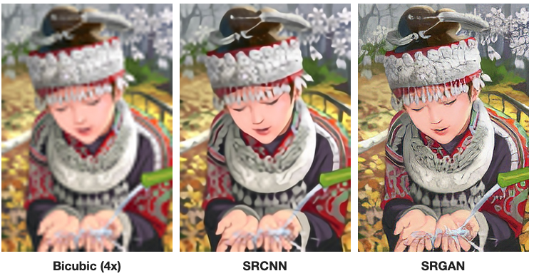
Fig 1. Image super-resolution techniques visual quality evolution.

To further enhance the visual quality of the images, ESRGAN architecture was introduced. The aim of this implementation was to reduce the often generated unpleasant artifacts from the hallucinated details created by the network. To further enhance the visual quality, Xintao et al. revisited the three key components of SRGAN: the network architecture, adversarial loss and perceptual loss; and improved each of them to derive to an Enhanced SRGAN (ESRGAN) network implementation.

First, they improved the network structure by introducing the novel Residual-in-Residual Dense Block (RRDB), which has higher capacity and is easier to train. They also removed the Batch Normalization (BN) layers as in EDSR, as they tend to bring artifacts to generated images. Another improvement to the network was to use residual scaling and smaller initialization to facilitate training a very deep neural network. Second, they improved the discriminator by using a Relativistic average GAN (RaGAN) model, which learns to judge “whether one image is more realistic than the other” rather than “whether one image is real or fake”. Third, they propose an improved perceptual loss by using the VGG features before activation instead of after activation as in SRGAN. Furthermore, in order to balance the visual quality and RMSE/PSNR, a network interpolation strategy is suggested, which could continuously adjust the reconstruction style and smoothness.

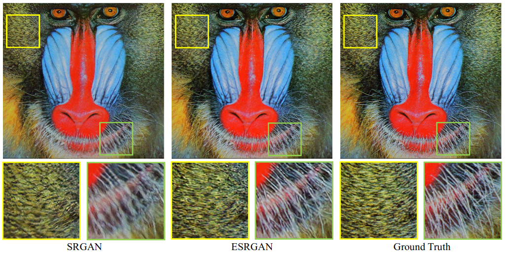
Fig 2. Comparison of single image super-resolution between SRGAN and ESRGAN implementations.

To top

2. Motivation

The aim of choosing a project based on single image super-resolution was to investigate the current existing set of deep-learning techniques because of the wide range of possible solutions to real challenges that they can provide.

Following our project advisor’s recommendations, we decided to follow the Generative Adversarial network-based SR approach, which represented a great opportunity to learn more about this kind architectures. Training a GAN network is a nice challenge given the complexity of having to train two different networks competing with each to outperform and fool the system.

As mentioned previously, the idea of the project was to target a solution with potential appliance at business level.

To top

3. Execution instructions

asdf asdf

3.1 Installation

You can install torch-sr via pip or directly from source.

Install from GitHub

You can install the latest development version using pip directly from the GitHub repository:

pip install git+https://github.com/AIDL-PROJ-2022/enhanced-srgan.git

Install from source

It's also possible to clone the Git repository and install it from source using pip:

git clone https://github.com/AIDL-PROJ-2022/enhanced-srgan.git
cd enhanced-srgan
pip3 install -r requirements.txt

3.2 ESRGAN model training

Model can be trained using the train.py script that can be found on the root project directory.

usage: train.py [-h] [-l LOAD_CHECKPOINT] [-a] [--no-data-parallel] [-i CHECKPOINT_INTERVAL] [-w BEST_CHECKPOINT_WARMUP] [-s STORE_MODEL_INTERVAL] config_file

positional arguments:
  config_file           JSON training configuration hyper-parameters

optional arguments:
  -h, --help            show this help message and exit
  -l LOAD_CHECKPOINT, --load-checkpoint LOAD_CHECKPOINT
                        Path to the training checkpoint used as the start point
  -a, --autocast        Use PyTorch autocast when running on GPU with CUDA support
  --no-data-parallel    Disable parallelization if more than one GPU is detected on the system
  -i CHECKPOINT_INTERVAL, --checkpoint-interval CHECKPOINT_INTERVAL
                        Define checkpoint store frequency. Default: 1
  -w BEST_CHECKPOINT_WARMUP, --best-checkpoint-warmup BEST_CHECKPOINT_WARMUP
                        Define a warm-up period until best checkpoint is stored. Default: 0
  -s STORE_MODEL_INTERVAL, --store-model-interval STORE_MODEL_INTERVAL
                        Define model store frequency. If not specified, model won't be stored during training.

By default, all model checkpoints and state dictionaries will be stored to saved_models/ directory relative to the working directory.

Example

python train.py --config-json configs/esrgan_192_cr_23_rrdb_div2k.json --load-model-path saved_models/1657192860_RRDB_PSNR_x4_best_model.pth --autocast --best-checkpoint-warmup 2000 --store-model-interval 20 --checkpoint-interval 50

3.3 ESRGAN model test

Model can be tested using the test.py script that can be found on the root project directory.

usage: test.py [-h] [-d DATASETS] [-s SHOW_RESULTS] [-o OUT_DIR] model_path

positional arguments:
  model_path            ESRGAN model path to test

optional arguments:
  -h, --help            show this help message and exit
  -d DATASETS, --datasets DATASETS
                        Datasets to use to test the specified model. Datasets need to be specified sepparated by a coma.
                        Example: --datasets=set5,set14. Available values are: 'div2k', 'bsds500', 'set5', and 'set14'.
  -s SHOW_RESULTS, --show-results SHOW_RESULTS
                        Show N best PSNR of all tested images. If not specified, only metrics will be plotted to terminal.
  -o OUT_DIR, --out-dir OUT_DIR
                        Specify output directory where all results will be stored. If not specified, results won't be stored.

Example

python3 test.py --datasets=set5 --out-dir results/192_cr_23_rrdb_div2k/set5 models/192_cr_23_rrdb_div2k/RRDB_ESRGAN_x4.pth

3.4 ESRGAN model inference

Model inference can be run using the inference.py script that can be found on the root project directory. When running inference, super-resolution can be applied to custom user-provided images and store the results.

usage: inference.py [-h] -m MODEL_PATH [-o OUT_DIR] images [images ...]

positional arguments:
  images

optional arguments:
  -h, --help            show this help message and exit
  -m MODEL_PATH, --model-path MODEL_PATH
                        Input generator model path. Can be a checkpoint or a final model.
  -o OUT_DIR, --out-dir OUT_DIR
                        Output directory where inferred images will be stored. If not specified, resultant images will 
                        be stored to the same directory from where they were found.

To differentiate original from super-resolved images, the _sr suffix will be appended to each input image name.

Example

python3 inference.py --model-path models/192_cr_23_rrdb_div2k/RRDB_ESRGAN_x4.pth ~/Pictures/my-fancy-picture.png

3.5 ESRGAN network interpolation

The script net_interpolation.py can be used to perform network interpolation as described in Network Interpolation.

usage: net_interpolation.py [-h] --psnr-model-path PSNR_MODEL_PATH --esrgan-model-path ESRGAN_MODEL_PATH --alpha ALPHA out_model_path

positional arguments:
  out_model_path        Output interpolated model

optional arguments:
  -h, --help            show this help message and exit
  --psnr-model-path PSNR_MODEL_PATH
                        PSNR-based (pre-training) input model path.
  --esrgan-model-path ESRGAN_MODEL_PATH
                        ESRGAN-based (training) input model path.
  --alpha ALPHA         Network interpolation alpha.

Example

python3 net_interpolation.py --psnr-model-path models/128_cr_23_rrdb_div2k/RRDB_PSNR_x4.pth  models/128_cr_23_rrdb_div2k/RRDB_ESRGAN_x4.pth  --alpha 0.9 models/128_cr_23_rrdb_div2k/RRDB_ESRGAN_x4_0.9_interp.pth

To top

4. Milestones

The main milestones throughout this project were:

Project preparation.
Dataset Preparation & Loading.
First Model Training.
First metrics and model training.
Project Review and conclusions.

To top

5. Datasets

We are using two types of datasets

BSDS500
- Standard benchmark for edge and contour detection segmentation.
- Consists of 500 images, each with 5 different ground truth segmentations.
- Contains:
  - 200 images for training.
  - 100 images for validation.
  - 200 images for testing.
DIV2K
- Recommended for SR given the different types of degradations contained in this dataset.
- Different upscaling and downscaling steps applied to obtain those degradations.
- 1000 images. All with 2K resolution.
- Contains:
  - 800 images for training.
  - 100 images for validation.
  - 100 images for testing.
SET5
- The Set5 dataset is a dataset consisting of 5 images (“baby”, “bird”, “butterfly”, “head”, “woman”) commonly used for testing performance of Image Super-Resolution models.
SET14
- The Set14 dataset is a dataset consisting of 14 images commonly used for testing performance of Image Super-Resolution models.

To top

6. Environment

The project has been fully implemented using Pytorch Framework. Additionally, the Albumentations library has been included in order to perform the crops and different transformations to the images from the Dataset.

Most of the trials have been carried out within local environment because the availability of the equipment and the timing constraints that the project has faced.

Raul Puente's server:
- CPU: Intel(R) Core(TM) i9-10900F CPU @ 2.80GHz
- RAM: 64 GB
- GPU: GeForce® RTX 3070 - 4 GB RAM
Marc Bermejo's server:
- CPU: AMD Ryzen™ 9 3900X @ 3.8GHz
- RAM: 32 GB
- GPU: GeForce® GTX 1080 Ti - 11 GB RAM

Once the project reached an acceptable level of maturity, different trainings have been performed in a Google Cloud environment to improve network training speed and allow more parallel trainings.

Google cloud environment:
- GPU: NVIDIA V100 GPUs
- RAM: 30 GB
- CPU: 8 VIRTUAL CPU

In terms of data visualization and logging, both Wandb and Tensorboard have been included into the project given that W&B can support Tensorboard and each of them provides additional features. For example: Wandb allows tracking the images created after each epoch and Tensorboard displays the model Graph for each execution.

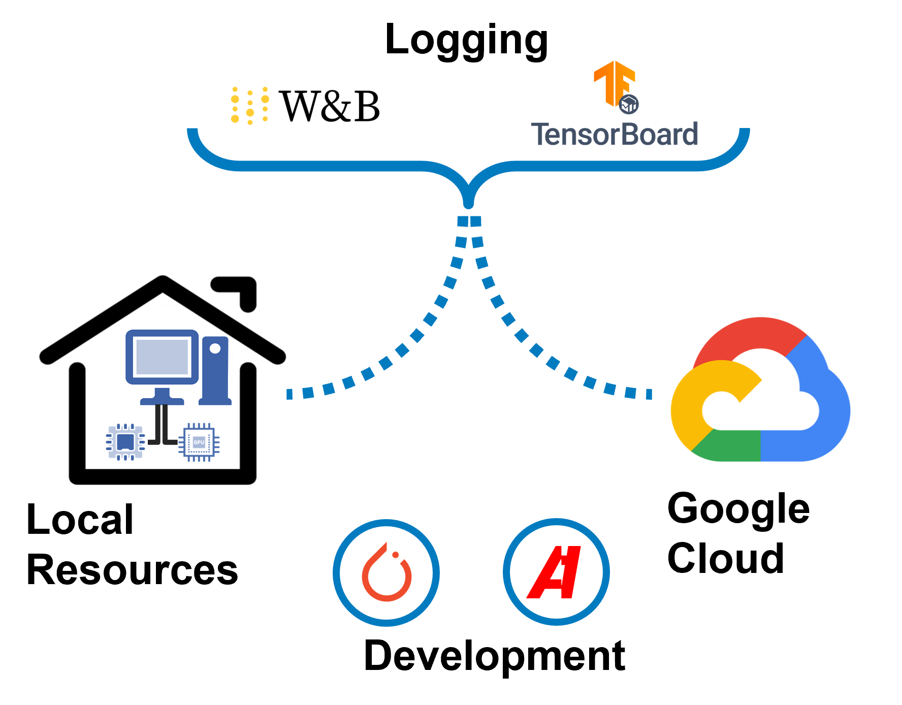
Fig 3. Model training execution environment diagram.

To top

7. Architecture

We've implemented a ESRGAN model using PyTorch

In this section we describe the proposed network architecture by the original ESRGAN implementation. This includes both generator and discriminator models definitions. Then we expose the available hyper-parameters that can be tuned to improve or modify the training process. After, we define the loss functions and quality metrics used to train and measure the model performance. At last, we describe the network interpolation process as described in the original paper.

7.1 Generator model

In order to further improve the recovered image quality of SRGAN, two modifications are made to the structure of generator in respect to the SRGAN implementation G:

Remove all BN layers.
Replace the original basic block with the proposed Residual-in-Residual Dense Block (RRDB), which combines multi-level residual network and dense connections as depicted in Fig. 4.

Fig 4. Left: BN layers were removed from the residual block of SRGAN. Right: RRDB block is used in our deeper model and β is the residual scaling parameter.

Removing BN layers has proven to increase performance and reduce computational complexity in different PSNR-oriented tasks including SR and deblurring. BN layers normalize the features using mean and variance in a batch during training and use estimated mean and variance of the whole training dataset during testing. When the statistics of training and testing datasets differ a lot, BN layers tend to introduce unpleasant artifacts and limit the generalization ability.

As from the ESRGAN specification, they keep the high-level architecture design of SRGAN (see Fig. 5), and use a novel basic block namely RRDB as depicted in Fig. 4. Based on the observation that more layers and connections could always boost performance, the proposed RRDB employs a deeper and more complex structure than the original residual block in SRGAN. Specifically, as shown in Fig. 4, the proposed RRDB has a residual-in-residual structure, where residual learning is used in different levels.

In addition to the improved architecture, Xintao et al. also exploit several techniques to facilitate training a very deep network:

Residual scaling, i.e., scaling down the residuals by multiplying a constant between 0 and 1 before adding them to the main path to prevent instability.
Smaller initialization, as they empirically find residual architecture is easier to train when the initial parameter variance becomes smaller.

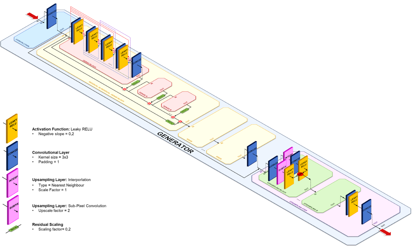
Fig 5. ESRGAN generator model diagram

7.2 Discriminator model

The discriminator model is a VGG-style network that will be trained and responsible of classifying the images between real and fake ones. It contains eight convolutional layers with an increasing number of 3x3 filter kernels, increasing by a factor of 2 from 64 to 512 kernels as in the VGG network. Strided convolutions are used to reduce the image resolution each time the number of features is doubled. The resulting 512 feature maps are followed by one dense layer of size 100, and a final perceptron that will act as the network binary classification output.

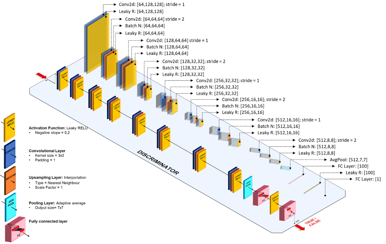
Fig 6. ESRGAN discriminator model diagram

7.3 Hyper-parameters

This table shows all the available network hyper-parameters that can be used to define a training process and network properties.

Hyperparameters	Default Values	Comments
scale_factor	`4`	Scale factor relation between the low resolution and the high resolution images.
batch_size	`16`	Data loader configured mini-batch size.
img_channels	`3`	Number of channels contained into the image. For RGB images this value should be 3.
pretraining/num_epoch	`10000`	Number of epoch needed to complete the pre-training (PSNR-driven) step.
pretraining/cr_patch_size	`[128, 128]`	High-resolution image crop size. Needs to be a tuple of (H, W). If set to None, any crop transform will be applied.
pretraining/lr	`2e-4`	Configured learning rate for the pre-training step optimizer. Adam optimizer will be used for this step.
pretraining/sched_step	`200000`	Learning rate scheduler decay rate for the pre-training step.
pretraining/sched_gamma	`0.5`	Multiplicative factor of the learning rate scheduler decay for the pre-training step.
pretraining/train_datasets	`["div2k"]`	Dataset(s) used during training of the pre-training step. Must be one of `'div2k'`, `'bsds500'`.
pretraining/val_datasets	`["div2k"]`	Dataset(s) used during validation of the pre-training step. Must be one of `'div2k'`, `'bsds500'`.
training/num_epoch	`8000`	Number of epoch needed to complete the training step.
training/cr_patch_size	`[128, 128]`	Number of epoch needed to complete the pre-training (GAN-driven) step.
training/g_lr	`1e-4`	Configured generator's learning rate for the training step optimizer. Adam optimizer will be used for this step.
training/d_lr	`1e-4`	Configured discriminator's learning rate for the training step optimizer. Adam optimizer will be used for this step.
training/g_sched_steps	`[50000, 100000, 200000, 300000]`	List of mini-batch indices learning rate decay of the generator's training scheduler.
training/g_sched_gamma	`0.5`	Multiplicative factor of the generator's learning rate scheduler decay for the training step.
training/d_sched_steps	`[50000, 100000, 200000, 300000]`	List of mini-batch indices learning rate decay of the discriminator's training scheduler.
training/d_sched_gamma	`0.5`	Multiplicative factor of the discriminator's learning rate scheduler decay for the training step.
training/g_adversarial_loss_scaling	`0.005`	Generator adversarial loss scaling factor used to calculate the total generator loss.
training/g_content_loss_scaling	`0.01`	Generator content loss scaling factor used to calculate the total generator loss.
training/train_datasets	`["div2k"]`	Dataset(s) used during training of the training step. Must be one of `'div2k'`, `'bsds500'`.
training/val_datasets	`["div2k"]`	Dataset(s) used during validation of the training step. Must be one of `'div2k'`, `'bsds500'`.
generator/rrdb_channels	`64`	Number of channels in the residual-on-residual dense blocks latent space.
generator/growth_channels	`32`	Number of channels in the residual dense block latent space.
generator/num_basic_blocks	`16`	Number of basic (a.k.a residual-on-residual dense blocks) of the generator network.
generator/num_dense_blocks	`3`	Number of residual dense blocks contained into each RRDB block.
generator/num_residual_blocks	`5`	Number of convolutional blocks contained into each residual dense block.
generator/residual_scaling	`0.2`	Scaling factor applied to each skip connection defined into the generator network.
generator/use_subpixel_conv	`false`	If set to `True`, a Sub-Pixel convolution block will be used for up-scaling instead of the original interpolation up-scaling block.
discriminator/vgg_blk_ch	`[64, 64, 128, 128, 256, 256, 512, 512]`	Tuple containing the output channels of each convolution of the network. If two consecutive convolutions have the same output channels, a stride of two will be applied to reduce feature map dimensions.
discriminator/fc_features	`[100]`	Fully connected hidden layers output dimension.
content_loss/loss_f	`"l1"`	Loss function to use to compute pixel-wise distance between images. Must be one of: `'l1'`, `'l2'`, `'mse'`.
perceptual_loss/layer_weights	`{"conv5_4": 1.0}`	The weight for each layer of the VGG network used for loss calculation.
perceptual_loss/vgg_type	`"vgg19"`	Type of VGG network used as the perceptual loss' feature extractor. Must be one of: `'vgg11'`, `'vgg13'`, `'vgg16'`, `'vgg19'`.
perceptual_loss/criterion	`"l1"`	Loss function to compute distance between features. Must be one of: `'l1'`, `'l2'`.
perceptual_loss/normalize_input	`true`	If set to `True`, normalize the input image before doing inference though the VGG network. The mean and standard deviation values are calculated for an image in the range `[0, 1]`.
perceptual_loss/normalize_loss	`false`	If set to `True`, divide the total perceptual loss by the sum of the specified layers weight.

To top

7.4 Loss functions

Whe have 3 kind of loss functions on this model.

7.4.1 Content loss

The content loss ($L_{content}$) is used to evaluate the 1-norm distances between recovered image G($x_i$) and the ground-truth image $y_i$. Can be configured to use the L1 (Mean Absolute Error) or L2 (Mean Square Error) function. By default, we use L1 function.

Formulas:

$$ \begin{aligned} L1 = MAE = {SAE \over N} = {1 \over N} \sum_{t = 1}^{N} |y_t - f_t| \end{aligned} $$

$$ \begin{aligned} L2 = MSE = {SSE \over N} = {1 \over N} \sum_{t = 1}^{N} (y_t - f_t)^2 \end{aligned} $$

7.4.2 Relativistic adversarial loss

We use the relativistic GAN which tries to predict the probability that a real image $x_r$ is relatively more realistic than a fake one $x_f$, as shown in Fig. 7.

Fig 7. Difference between standard discriminator and relativistic discriminator.

where σ is the sigmoid function and C(x) is the non-transformed discriminator output and E$x_f$[·] represents the operation of taking average for all fake data in the mini-batch. The discriminator loss is then defined as:

$$ \begin{aligned} L_{D}^{Ra} = −E_{x_r} [log(D_{Ra}(x_r , x_f ))] − E_{x_f} [log(1 − D_{Ra}(x_f , x_r ))] \end{aligned} $$

And the adversarial los for generator is in a symmetrical form:

$$ \begin{aligned} L_{G}^{Ra} = −E_{x_r} [log(1 − D_{Ra}(x_r, x_f ))] − E_{x_f} [log(D_{Ra}(x_f , x_r ))] \end{aligned} $$

where $x_f = G(x_i)$ and $x_i$ stands for the input LR image.

7.4.3 Perceptual loss

The perceptual loss ($L_{percep}$): Type of content loss introduced in the Perceptual Losses for Real-Time Style Transfer and Super-Resolution framework. Also known as VGG loss is based on the ReLU activation layers on the pre-trained 19 layer VGG network.

$$ \begin{aligned} l_{VGG/i,j} = {1 \over W_{i,j}H_{i,j}} \sum_{x = 1}^{W_{i,j}} \sum_{y = 1}^{H_{i,j}} (\Phi_{i,j}(I^{HR}){x,y} - \Phi{i,j}(G_{\Phi_G}(I^{LR}))_{x,y})^2 \end{aligned} $$

but with the improvement of using VGG features before activation instead of after activation as in SRGAN. It was empirically found hat the adjusted perceptual loss provides sharper edges and more visually pleasing results.

7.4.4 GAN-driven generator loss

The total loss of the generator ($L_G$) during the GAN-driven training stage is then calculated by:

$$ \begin{aligned} L_G = L_{percep} + λL_{G}^{Ra} + ηL_{content} \end{aligned} $$

where λ, η are the coefficients to balance the different loss terms.

7.5 Quality Metrics

7.5.1 Structural Similarity Index (SSIM)

Given 2 images, SSIM is an index with values in the range (-1,1) which estimates the level of similarity between those two images. The value range will show the following behaviour:

+1 -> very similar or the same.
-1 -> very different.

It combines different comparison functions:

Luminance l(x,y).
Contrast c(x,y)
Structure s(x,y)

Formula:

$$ \begin{aligned} SSIM(x,y) = [l(x,y)]^α * [c(x,y)]^β * [s(x,y)]^γ \end{aligned} $$

Where α, β, γ are the weights assigned to each feature.

7.5.2 Peak Signal-to-Noise (PSNR)

Ratio between maximum possible value (power) of a signal and power of distorting noise that affects the quality of its representation.

Metric used to compare different image enhancement algorithms systematically to evaluate which produces better results using the same dataset.

Formula:

$$ \begin{aligned} PSNR = 20log_{10}({MAX_f\over\sqrt{MSE}}) \end{aligned} $$

Where MSE is the L2 loss and $MAX_f$ is the maximum existing signal value in our original “known to be good” image.

7.6 Network Interpolation

To remove unpleasant noise in GAN-based methods while maintain a good perceltual quality, we use Network Interpolation. That means that we first train a PSNR-oriented network $G_{PSNR}$ and then obtain a GAN-based network $G_{GAN}$.

We interpolate all the corresponding parameters of these two networks to derive an interpolated model $G_{INTERP}$, whose parameters are:

$$ \begin{aligned} θ_G^{INTERP} = (1 − α)θ_G^{PSNR} + αθ_G^{GAN} \end{aligned} $$

where $θ_G^{INTERP}$, $θ_G^{PSNR}$ and $θ_G^{GAN}$ are the parameters of $G_{INTERP}$, $G_{PSNR}$ and $G_{GAN}$ respectively, and α ∈ [0, 1] is the interpolation parameter.

To top

8. Training process

Training process is composed in two main steps, pre-traing (warm-up) and training.

First, in order to retrieve the dataset images, we perform the pipeline described in Fig 6:

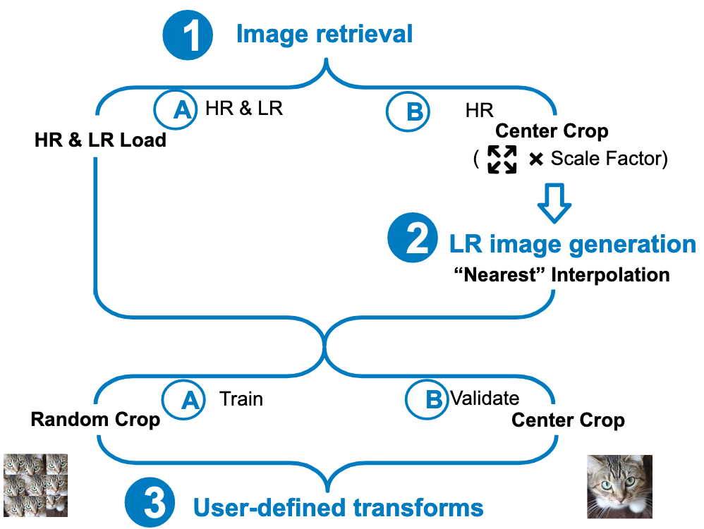
Fig 6. Image Retrieval Pipeline

As user-defined transforms we define the following ones depending on the augmentation target:

Spatial transforms.
- Applied for images of low resolution and high resolution.
- One of with 0.5 probability:
  - Flip with 0.25 probability.
  - Transpose with 0.75 probability.
Hard transforms:
- Applied only for images of low resolution.
- Compression with 0.25 probability.
- Coarse Dropout with 0.25 probability.

8.1 Pre-training step

In this step only the generator is trained using the Content loss as the loss function.

Only used the Content loss function for this step.
Only works with generator (no discriminator used).
Adam optimizer with learning rate $2e^{-4}$ by default.
Scheduler StepLR with step 175000 and gamma 0.5.
User data augmentation transforms:
- Spatial transforms.
- Hard transforms.
Metrics logged:
- Training: content_loss
- Validation: content_loss, perceptual_loss, PSNR, SSIM

8.2 Training step

In this step we train with generator and discriminator. For every mini batch we first freeze the discriminator and train the generator. When finished the mini batch then we train the discriminator and freeze the generator.

Generator:
- The total loss function is used for training the generator in this step, which is a combination of the perceptual loss, relativistic adversarial loss and content loss with scaling.
- Adam optimizer with learning rate $1^{e-4}$ by default and betas=(0.9, 0.99).
- Scheduler MultiStepLR with steps [50000, 100000, 175000, 250000] and gamma 0.5.
Discriminator:
- The relativistic adversarial loss function is used for discriminator in this step.
- Adam optimizer with learning rate $1^{e-4}$ by default and betas=(0.9, 0.99).
- Scheduler MultiStepLR with steps [50000, 100000, 175000, 250000] and gamma 0.5.
User data augmentation transforms:
- Spatial transforms.
Metrics logged:
- Training: content_loss, perceptual_loss, g_adversarial_loss, g_total_loss, d_adversarial_loss
- Validation: content_loss, perceptual_loss, PSNR, SSIM

8.3 Logging

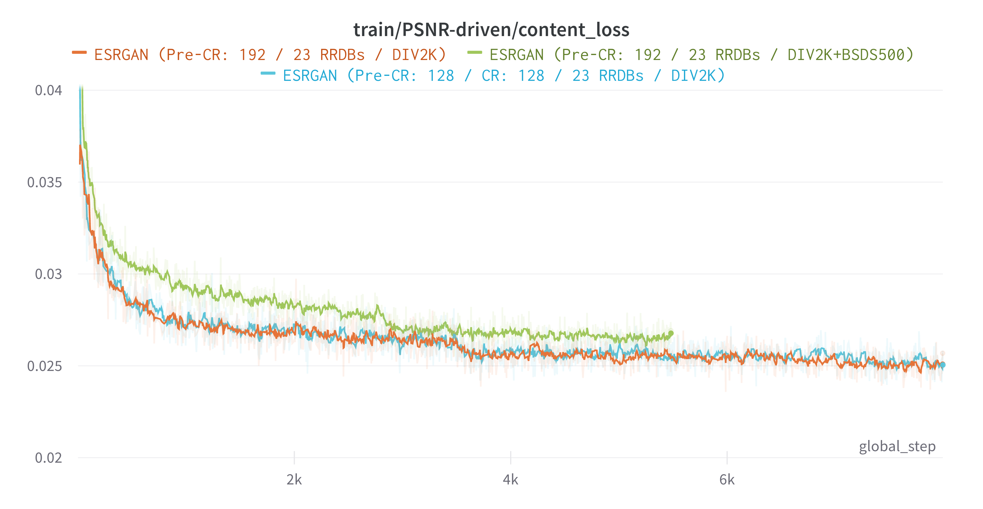
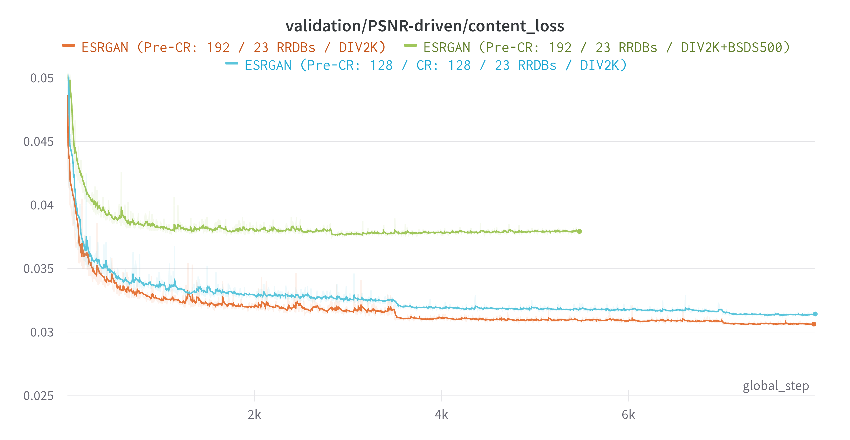
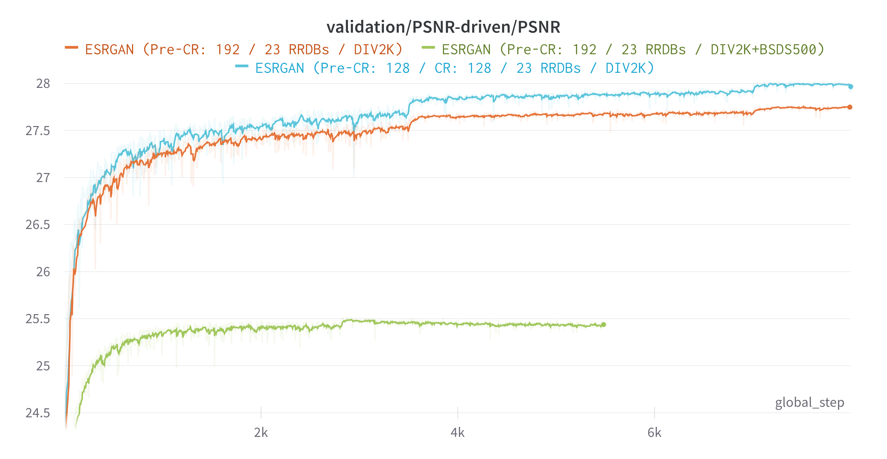
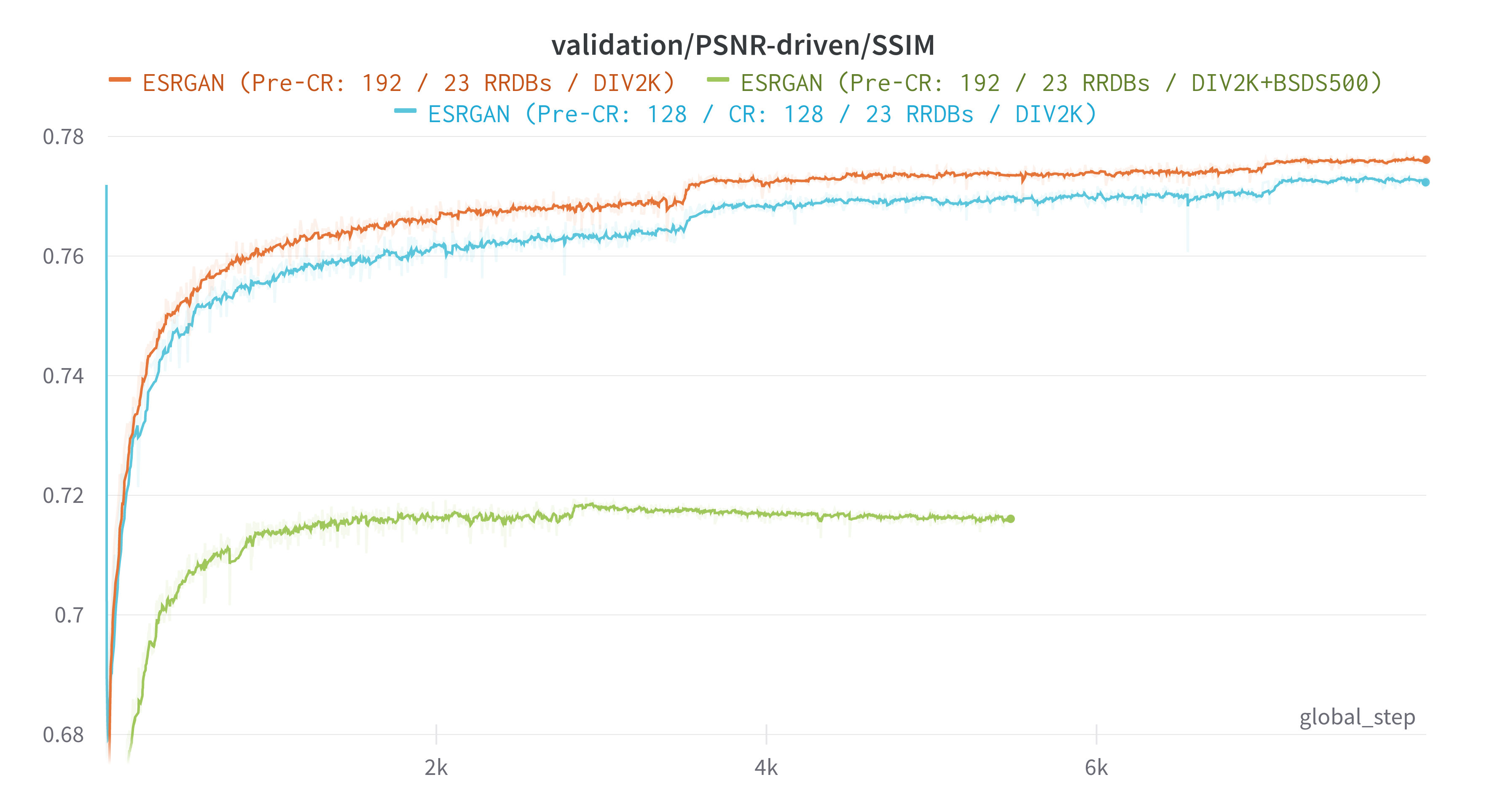
For logging we use wandb with Tensorboard integrated because we can work with both system and share all the logging information automatically to everyone and in real time. Besides, we upload images with the result of the image and the ground truth to compare the results visually for every N epochs.

To top

9. Results

9.1 Executions

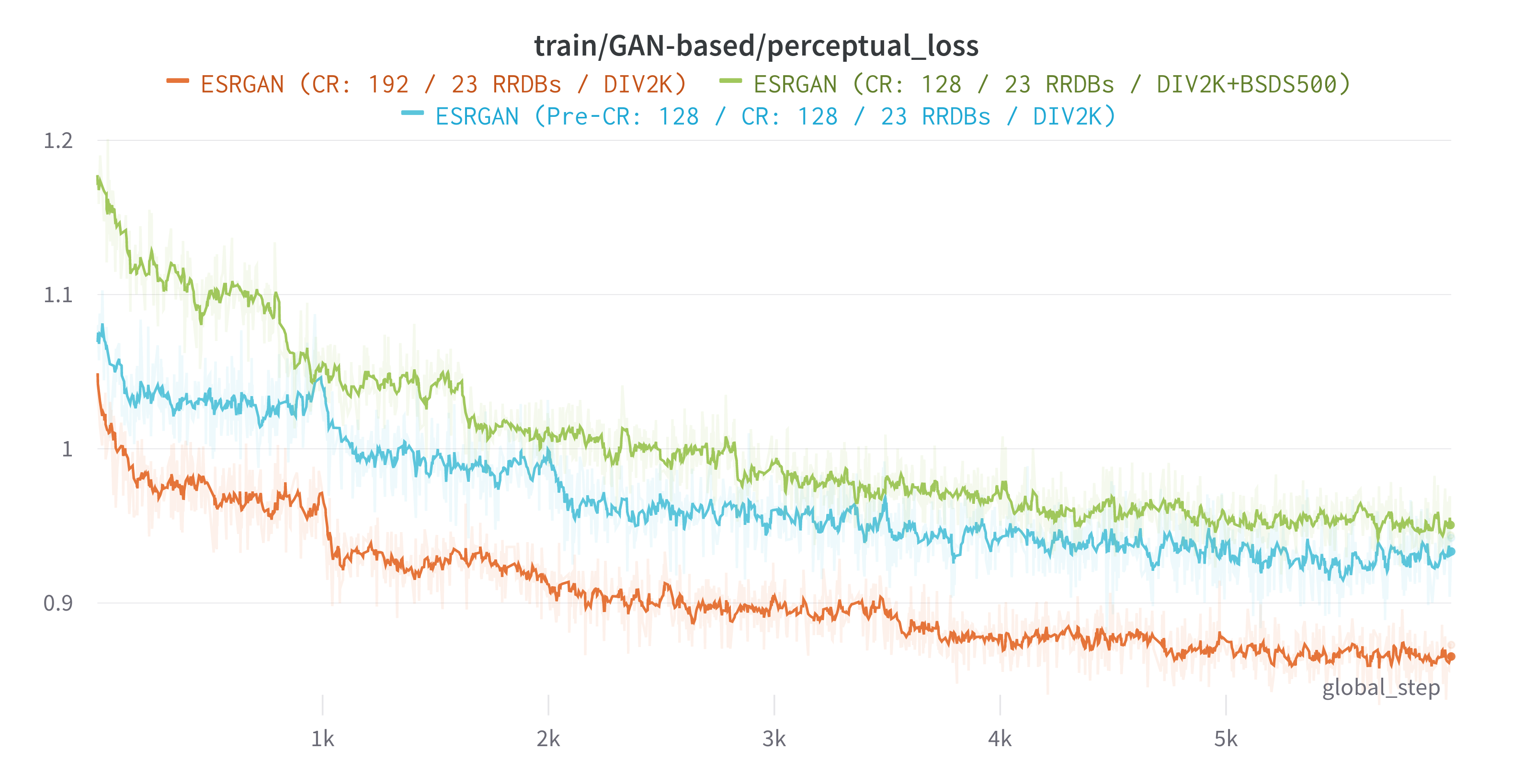
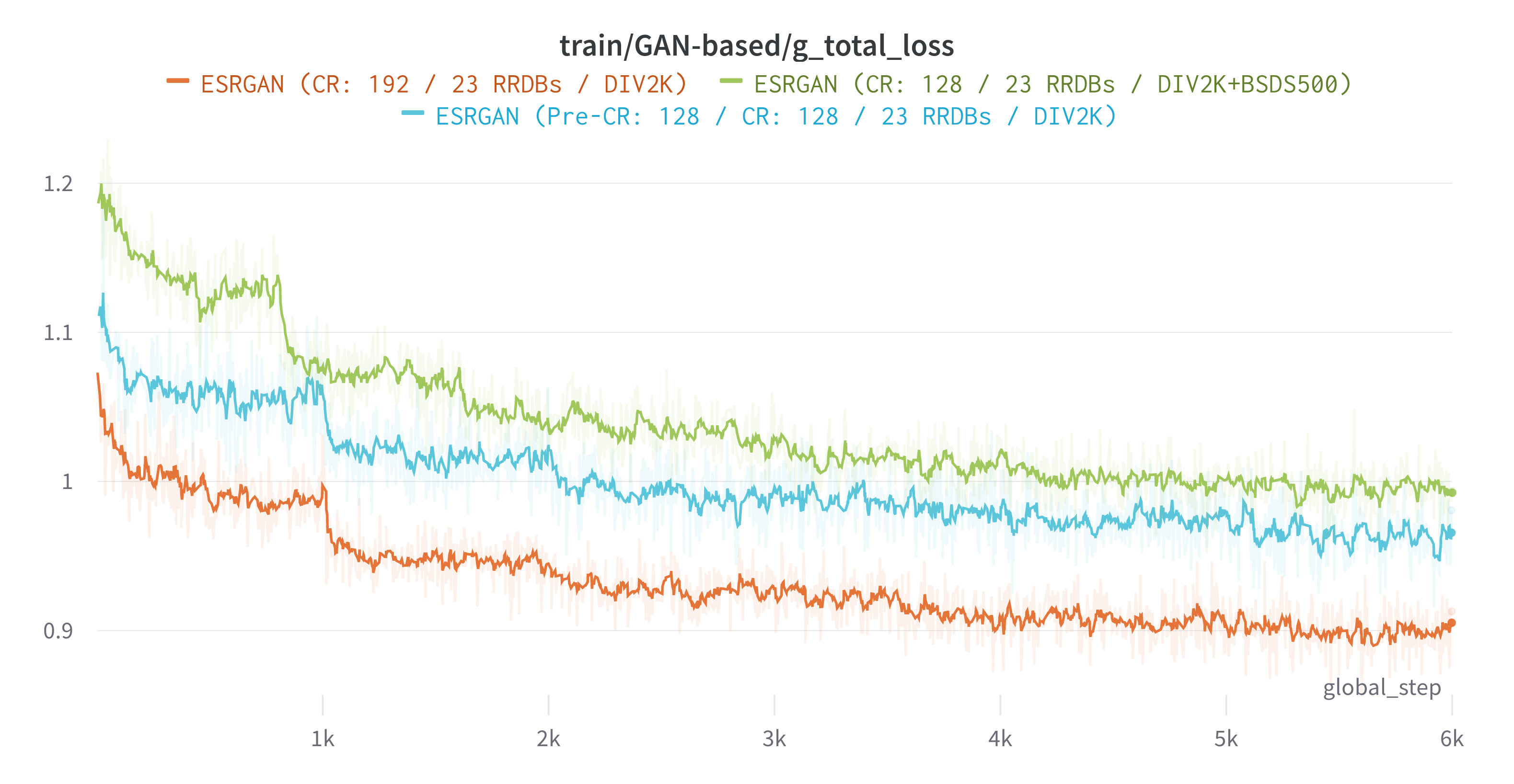
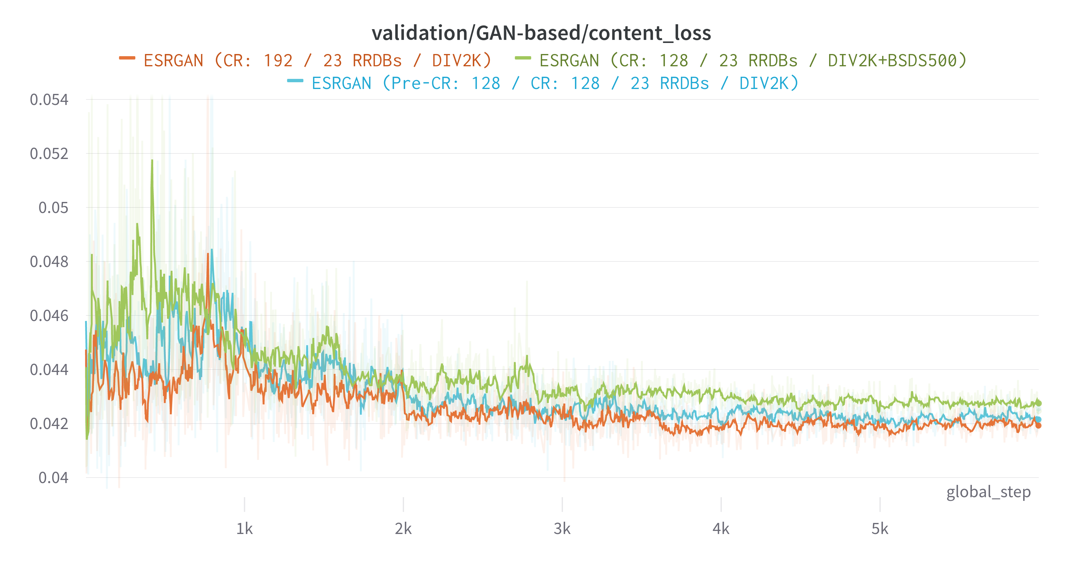
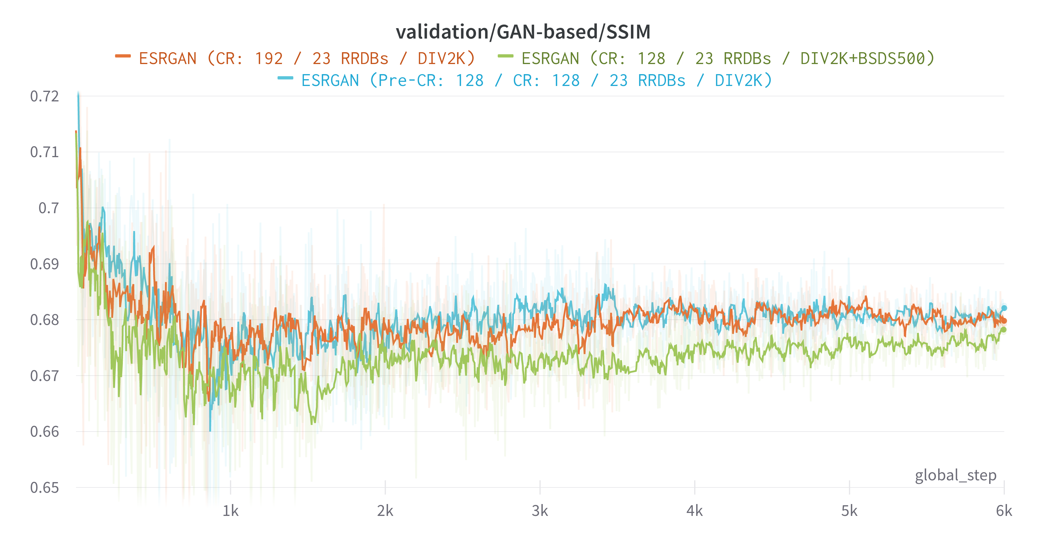
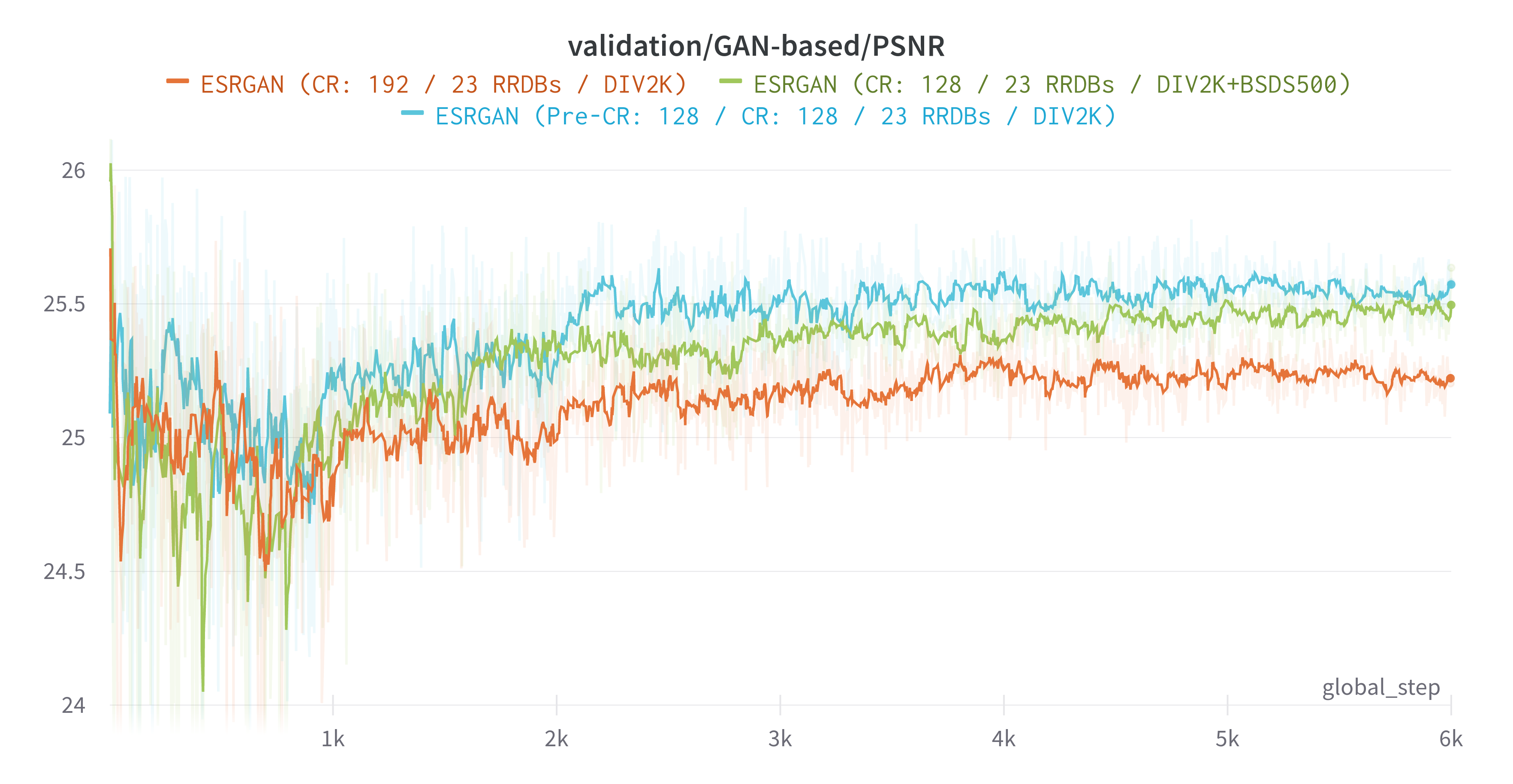
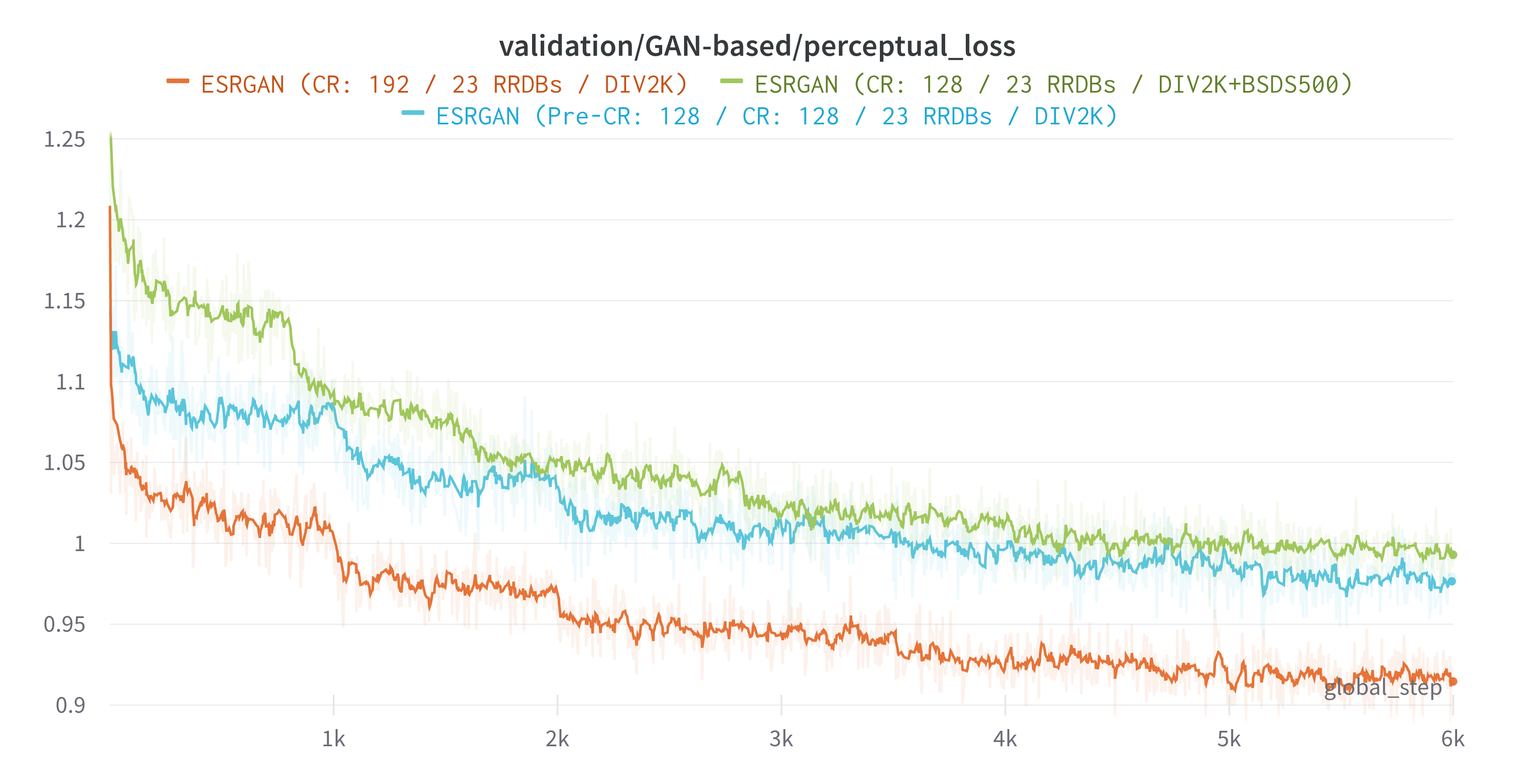
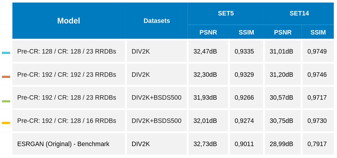
We have successfully completed 4 different executions with different hyper-parameters:

The trainings are described using the following structure:

PRE CR: Crop size used during the pre-training step.
CR: Crop size used during the training step.
RRDBs: Number of Residual-in-Residual dense block defined in the generator.
DIV2K / DIV2K+BSDS500: Datasets used during for training the model.

These are the hyper-parameters defined for each training:

ESRGAN (PRE CR: 128 / CR: 128 / 23 RRDBs / DIV2K)
- Wandb information pretraining and training
- Hyperparameters:
  - pretraining/cr_patch_size: [128, 128]
  - training/cr_patch_size: [128, 128]
  - generator/num_basic_blocks: 23
  - pretraining/train_datasets: ["div2k"]
  - training/train_datasets: ["div2k"]
ESRGAN (PRE CR: 192 / CR: 128 / 23 RRDBs / DIV2K+BSDS500)
- Wandb:
  - Wandb information pretraining
  - Wandb information training
- Hyperparameters:
  - pretraining/cr_patch_size: [192, 192]
  - training/cr_patch_size: [128, 128]
  - generator/num_basic_blocks: 23
  - pretraining/train_datasets: ["div2k", "bsds500"]
  - training/train_datasets: ["div2k", "bsds500"]
ESRGAN (PRE CR: 192 / CR: 192 / 23 RRDBs / DIV2K)
- Wandb:
  - Wandb information pretraining
  - Wandb information training
- Hyperparameters:
  - pretraining/cr_patch_size: [192, 192]
  - training/cr_patch_size: [192, 192]
  - generator/num_basic_blocks: 23
  - pretraining/train_datasets: ["div2k"]
  - training/train_datasets: ["div2k"]
ESRGAN (PRE CR: 192 / CR: 128 / 16 RRDBs / DIV2K+BSDS500)
- Wandb:
  - No data available for this training.
- Hyperparameters:
  - pretraining/cr_patch_size: [192, 192]
  - training/cr_patch_size: [128, 128]
  - generator/num_basic_blocks: 16
  - pretraining/train_datasets: ["div2k", "bsds500"]
  - training/train_datasets: ["div2k", "bsds500"]

From these trainings we wanted to confirm the following hypothesis:

The network will benefit from having a deeper structure and will achieve better results.
The network will achieve more generalization by using dataset with different semantics.
The network will be able to capture more spatial data from having a bigger crop.

9.2 Metrics

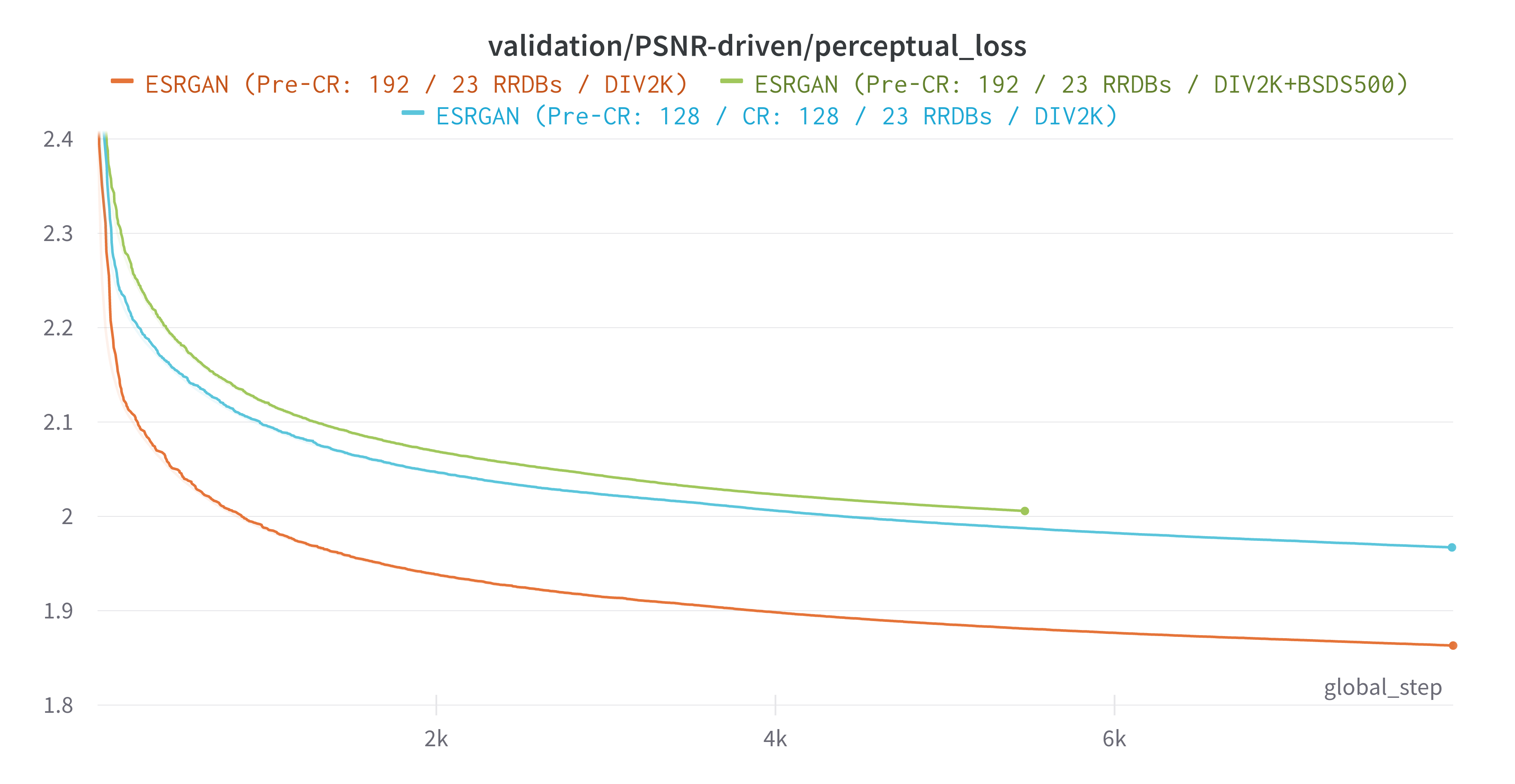
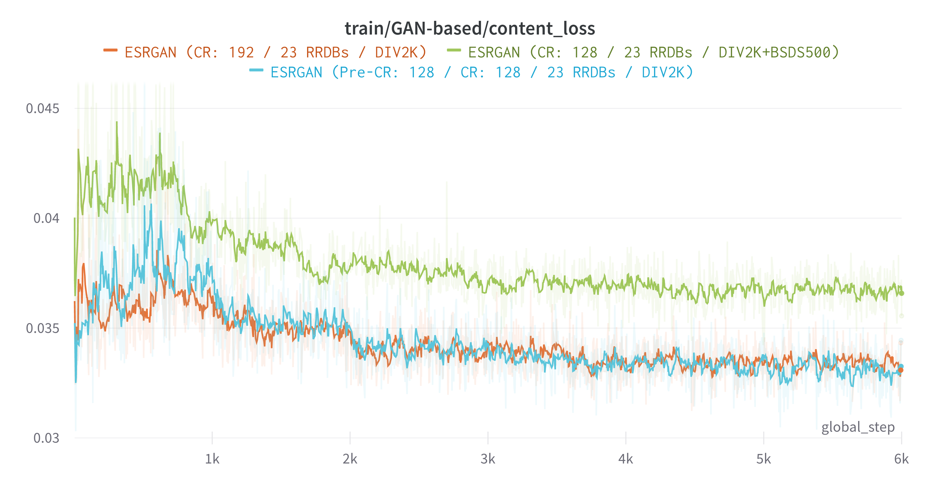
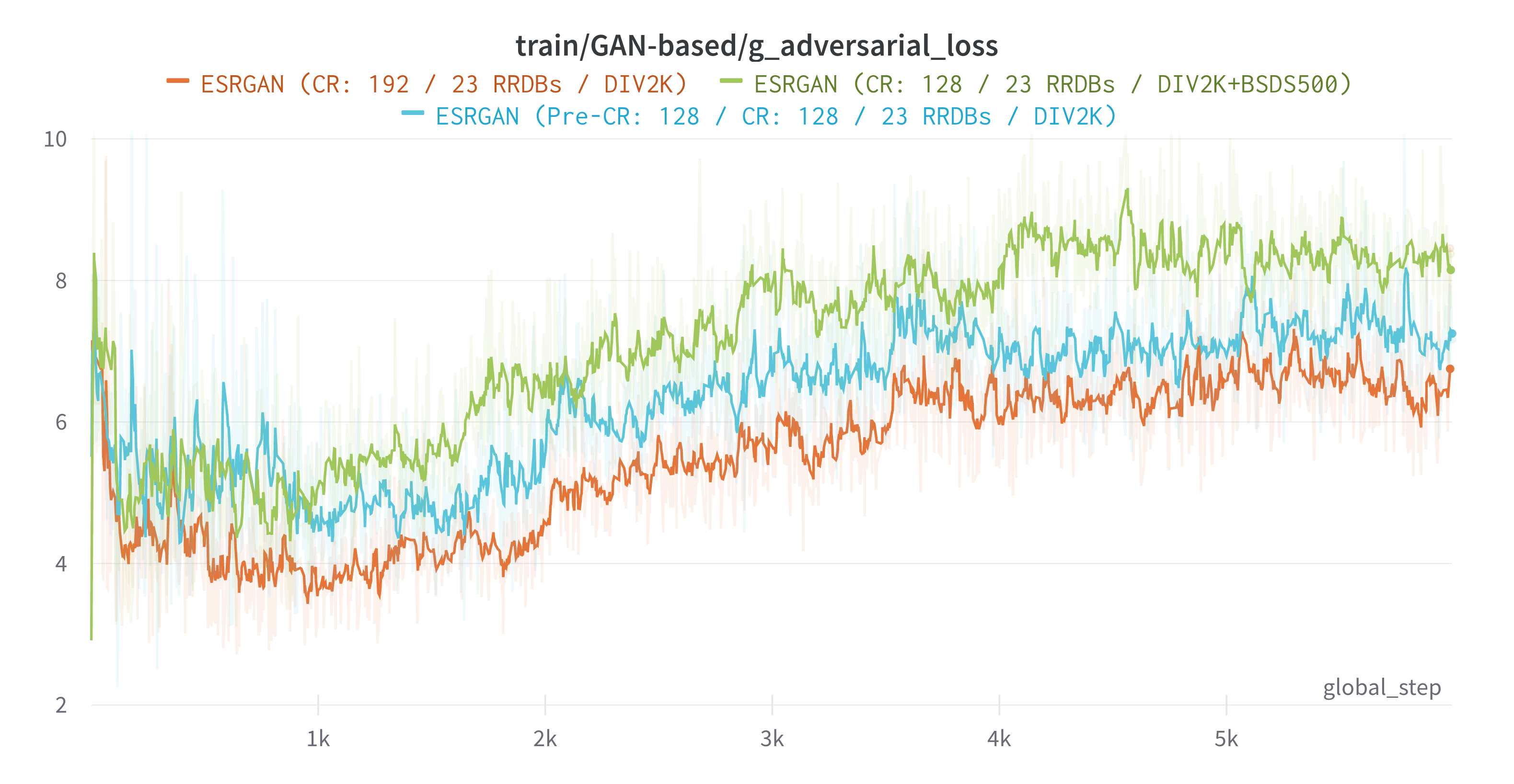
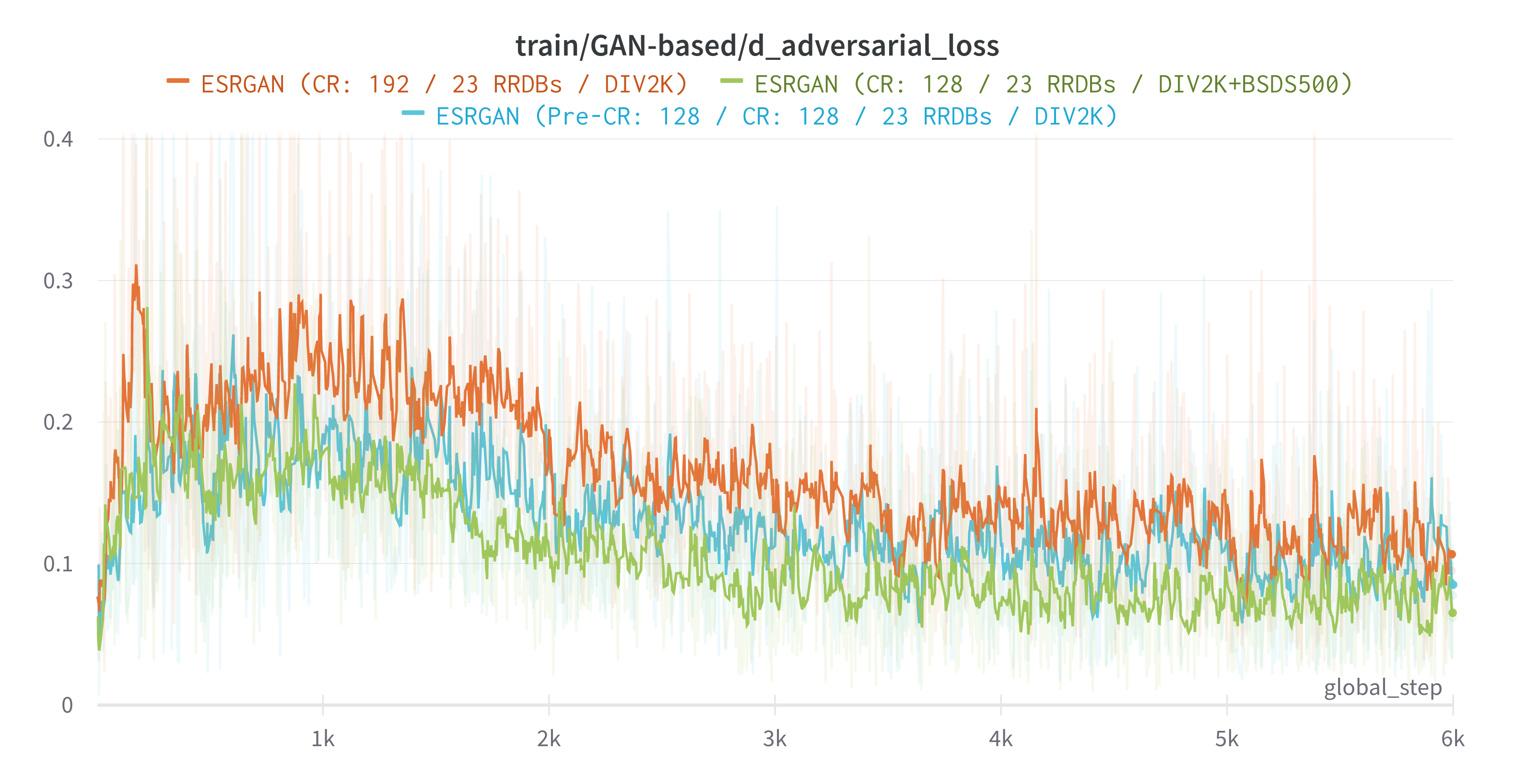
These are the metrics obtained from all steps and executed trainings.

9.2.1 Train (PSNR-driven)

9.2.2 Validation (PSNR-driven)

9.2.3 Train (GAN-based)

9.2.4 Validation (GAN-based)

9.3 Model Results

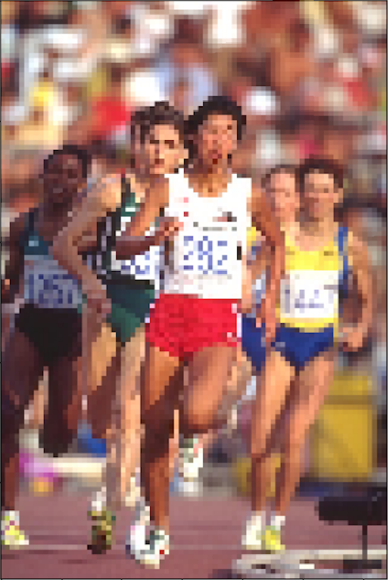
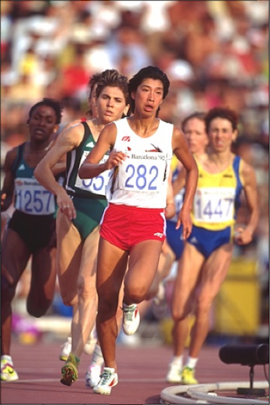
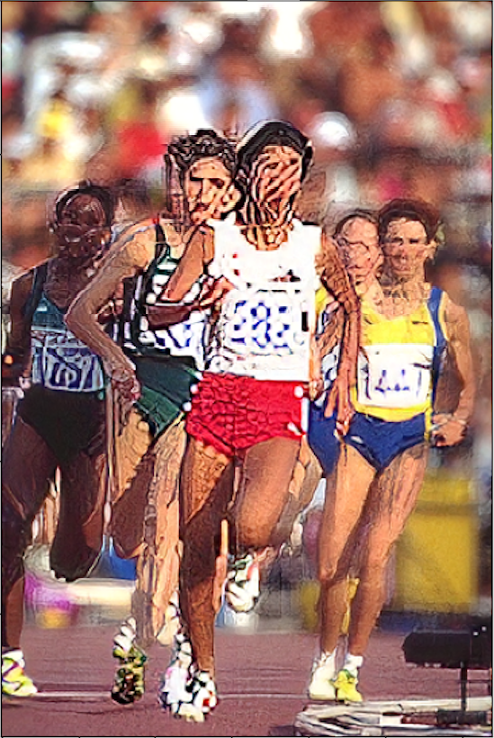
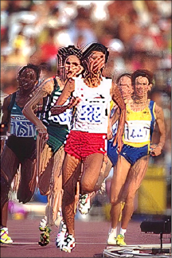
These are the results from some images of the SET5 and SET14 test datasets.

9.3.1 Butterfly

Low resolution	Ground Truth

Pre-CR: 128 / CR: 128 / 23 RRDBs / DIV2K	Pre-CR: 192 / CR: 192 / 23 RRDBs / DIV2K

PSNR: 25.97db / SSIM: 0.87	PSNR: 26.4ldb / SSIM: 0.88

Pre-CR: 192 / CR: 128 / 16 RRDBs / DIV2K+BSDS500	Pre-CR: 192 / CR: 128 / 23 RRDBs / DIV2K+BSDS500

PSNR: 25.96db / SSIM: 0.88	PSNR: 26.1ldb / SSIM: 0.88

9.3.2 Parrot

Low resolution	Ground Thruth

Pre-CR: 128 / CR: 128 / 23 RRDBs / DIV2K	Pre-CR: 192 / CR: 192 / 23 RRDBs / DIV2K

PSNR: 32.47db / SSIM: 0.9	PSNR: 32.3db / SSIM: 0.9

Pre-CR: 192 / CR: 128 / 16 RRDBs / DIV2K+BSDS500	Pre-CR: 192 / CR: 128 / 23 RRDBs / DIV2K+BSDS500

PSNR: 32.02db / SSIM: 0.9	PSNR: 31.93db / SSIM: 0.9

9.3.3 Runners

Low resolution	Ground Thruth

Pre-CR: 128 / CR: 128 / 23 RRDBs / DIV2K	Pre-CR: 192 / CR: 192 / 23 RRDBs / DIV2K

PSNR: 16.18db / SSIM: 0.44	PSNR: 16.44db / SSIM: 0.45

Pre-CR: 192 / CR: 128 / 16 RRDBs / DIV2K+BSDS500	Pre-CR: 192 / CR: 128 / 23 RRDBs / DIV2K+BSDS500

PSNR: 20.12db / SSIM: 0.66	PSNR: 20.37db / SSIM. 0.67

To top

9.4 Torch Models pre-trained

Model	Download	Comments
p192_t128_cr_23_rrdb_div2k+bsds500	PSNR.pth	PSNR model
p192_t128_cr_23_rrdb_div2k+bsds500	ESRGAN.pth	ESRGAN model
p192_t128_cr_23_rrdb_div2k+bsds500	ESRGAN-interp.pth	ESRGAN model interpolated with alpha=0.8
p192_t128_cr_16_rrdb_div2k+bsds500	PSNR.pth	PSNR model
p192_t128_cr_16_rrdb_div2k+bsds500	ESRGAN.pth	ESRGAN model
p192_t128_cr_16_rrdb_div2k+bsds500	ESRGAN-interp.pth	ESRGAN model interpolated with alpha=0.8
p192_cr_23_rrdb_div2k	PSNR.pth	PSNR model
p192_cr_23_rrdb_div2k	ESRGAN.pth	ESRGAN model
p192_cr_23_rrdb_div2k	ESRGAN-interp.pth	ESRGAN model interpolated with alpha=0.8
128_cr_23_rrdb_div2k	PSNR.pth	PSNR model
128_cr_23_rrdb_div2k	ESRGAN.pth	ESRGAN model
128_cr_23_rrdb_div2k	ESRGAN-interp.pth	ESRGAN model interpolated with alpha=0.8

To top

9.5 Comparison metrics

To top

10. Conclusions

It has been a very challenging project, and we have learned a lot. One of the first issues we faced is the hardware limitation. It took a lot of time to train the models, and the batch and crop sizes were limited directly by the available GPU memory.

After observing the obtained results we can extract the following conclusions:

During the GAN-based training is really important and difficult to maintain the balance between the generator and the discriminator training.
Using network interpolation we can reduce unpleasant noise from GAN-driven training while maintaining a good perceptual performance.
A deeper model can further improve recovered textures and reduce unpleasant noises.
Using broader data with different scene types and sizes can help the generator to generalize more but at the cost of reducing overall performance.
Using more data for each epoch will produce overfitting faster than expected during the pre-training stage.
To achieve good performance on a scene type first the model needs to be trained from images with a similar semantics.
Using a dataset with sharper edges (like BSDS500) can help the network to perform better on images with less initial information and reduce generated images artifacts at the cost of reducing overall performance for easier images.

To top