`melt` project: comparing ice shelf melt models

Intercomparison of different models of basal melt

Models considered:

Simple: simple parametrizations based on thermal driving, i.e. difference between pressure freezing temperature and in-situ ocean temperature (e.g. Favier et al. (2019))
Plume: analytical approximtation of the 1D plume model (Lazeroms et al. (2019))
PICO: box model of cavity circulation (Reese et al. (2018))
PICOP: combination the two abovementioned models (Pelle et al. (2019))
Layer: 2D (vertically integratd) plume model (Hellmer et al. (1989))

Example Ice Shelf: Totten Glacier

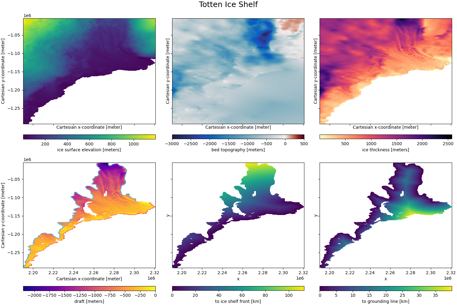
Figure 1: Geometry of the Totten Ice Shelf. The data in the top row is provided by the Bedmachine dataset. Left to right: surface elevation, bed topography/bathymetry, and ice thickness. Bottom left, derived draft of the ice shelf (elevation-thickness) together with the grounding line (blue) and the ice shelf front (red). Bottom center and right: minimum distance to the grounding line/ice shelf front.

Repository structure

melt
│   README.md
│   LICENSE
│
└───data
│   └───BedMachine           (Antarctic topography data; not committed here)
│   │   │   BedMachineAntarctica_2020-07-15_v02.nc
│   │
│   └───IceVelocity          (Radar derived surface velocities; not committed here)
│   │   │   antarctic_ice_vel_phase_map_v01.nc
│   │
│   └───mask_polygons        (polygons to select areas; created vi QGIS)
│       │   *_grl.geojson    (polygons around grounding lines, continent only)
│       │   *_grl2.geojson   (polygons around grounding lines, including islands)
│       │   *_isf.geojson    (polygons around ice shelf front)
│       │   *_polygon.geojson(polygons around whole ice shelf)
│
└───doc                      (documentation)
|   |   environment.yml      (conda environments file)
│
└───results                  (images & netcdf files, mostly not committed)
│   
└───src
    └───ipynb                (notebooks with output; not committed)
    │   │   BedMachineAntarctica_2020-07-15_v02.nc
    │
    └───notebooks            (notebooks without output; version controlled)
    │   │   example.ipynb    (recreate figure from README.md)
    │   │   ...
    │
    │   forcing.py        │
    │   ideal_geometry.py │  (set up model domains)
    │   real_geometry.py  │
    │   PICO.py         │
    │   PICOP.py        │
    │   Plume.py        │    (models)
    │   sheet.py        │
    │   Simple.py       │
    │   advect.py         │
    │   constants.py      │  (auxiliary functions)
    │   sheet_utils.py    │

How to run models

install the necessary packages
e.g., using conda env create -f environment.yml creates a conda environment named ice which should be able to execute all the code
choose geometry
```
from ideal_geometry import IdealGeometry
ds = IdealGeometry('test3').create()
```
realistic ice shelf geometries (with tht RealGeometry calss in real_geometry.py) require downloading the BedMachine topography and ice velocity data and placing it in the correct folder (see structure above)
choose forcing (temperature and salinity profiles)
```
from forcing import Forcing
pdict = dict(Tdeep=-2, ztcl=500)
ds = Forcing(ds).tanh(**pdict)
```
other forcing profiles are part of the Forcing class, including constant, tanh2, favier, isomip, isomipfrac, holland, holland07

pass those to model of choice

from Simple import SimpleModels
ds = SimpleModels(ds).compute()

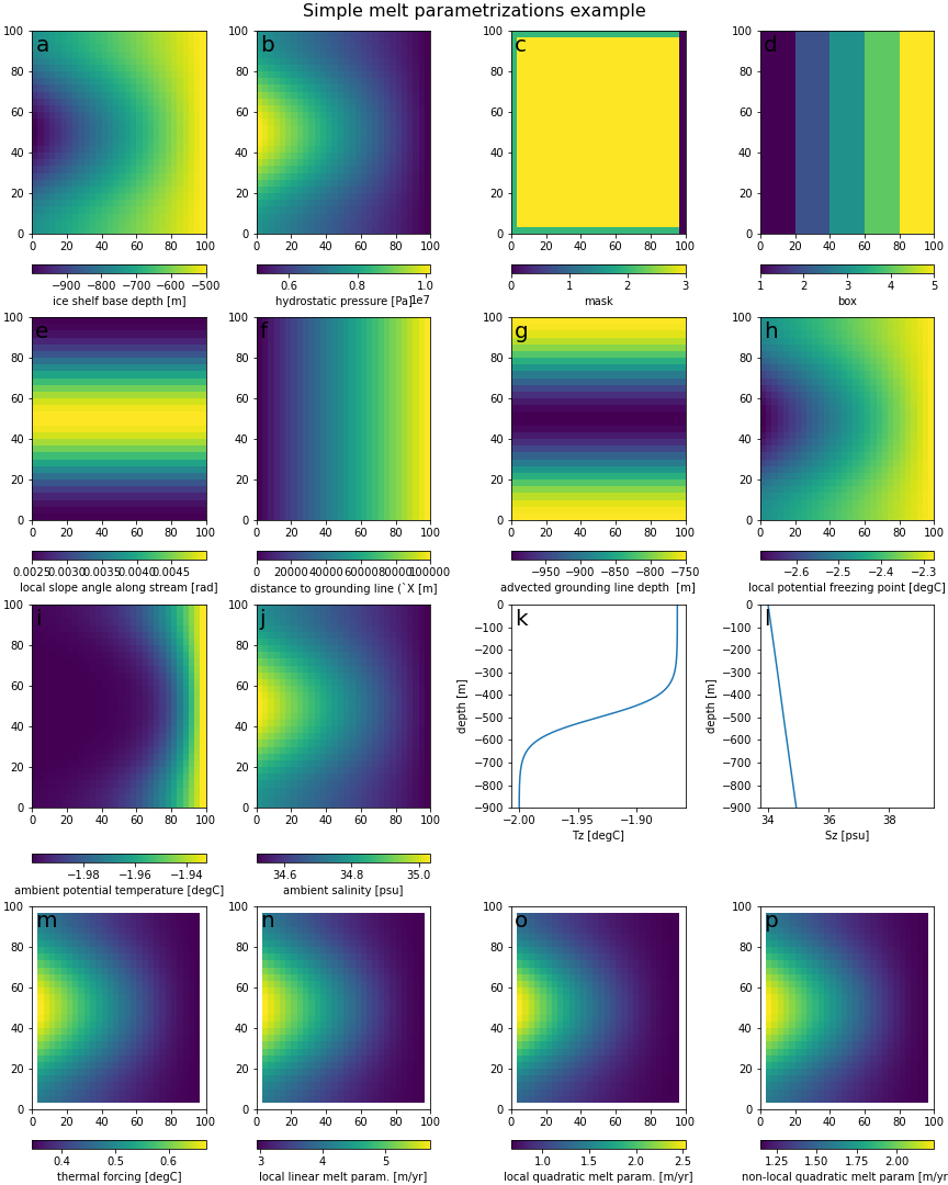
Figure 2: The results from following the example above: applying the Simple melt parametrizations on the test3 with a tanh forcing profile. The draft (a) is prescribed, the hydrostatic pressure (b) is linearly related, the mask (c) specifies grounding line (2), ice shelf (3), and ice shelf front (0), the number of boxes is given but the distribution (d) is calculated. Panels (e-g) show quantities needed for one or more melt model: the local slope angle along the flowline (here simply left to right), the distance to the grounding line, and the depth at the plume origin. Panel (h) shows the local freezing point, (i/j) the spatial distribution of temperature and salinity, (k/l) the temperature and salinity depth profiles. Panel (m) shows the thermal forcing (temperature minus local freezing point). Finally (n-p) show the three simple melt parameterizations: the local linear, local quadratic, and non-local quadratic ones, respectively

Disclaimer

This is work in progress and we do not guarantee anything. Contact us if you have questions, and if you find this useful also let us know.

References

Favier, Lionel et al. (June 2019a). “Assessment of sub-shelf melting parameterisations using the ocean–ice-sheet coupled model NEMO(v3.6)–Elmer/Ice(v8.3)”. Geoscientific Model Development 12.6., pp. 2255–2283.doi:10.5194/gmd-12-2255-2019.

Hellmer, H. H. and D. J. Olbers (Dec. 1989). “A two-dimensional model for the thermohaline circulation under an iceshelf”. Antarctic Science 1.4. pp. 325–336.issn: 1365-2079, 0954-1020. doi:10.1017/S0954102089000490

Lazeroms, Werner M.J. et al. (2019b). “An analytical derivation of ice-shelf basal melt based on the dynamics of meltwater plumes”. Journal of Physical Oceanography 49.4, pp. 917–939. doi:10.1175/JPO-D-18-0131.1

Pelle, Tyler, Mathieu Morlighem, and Johannes H. Bondzio (Apr. 2019a). “Brief communication: PICOP, a new ocean melt parameterization under ice shelves combining PICO and a plume model”. The Cryosphere 13.3. pp. 1043–1049. doi:10.5194/tc-13-1043-2019

Reese, Ronja et al. (June 2018a). “Antarctic sub-shelf melt rates via PICO”. The Cryosphere 12.6. pp. 1969–1985. doi:10.5194/tc-12-1969-2018.

AJueling/melt

melt project: comparing ice shelf melt models