


DiffEqFlux.jl fuses the world of differential equations with machine learning by helping users put diffeq solvers into neural networks. This package utilizes DifferentialEquations.jl and Flux.jl as its building blocks to support research in Scientific Machine Learning and neural differential equations in traditional machine learning.
- Problem Domain
- Citation
- Example Usage
- Use with GPUs
- Universal Differential Equations
- Neural Differential Equations for Non-ODEs: Neural SDEs, Neural DDEs, etc.
- API Documentation
- Benchmarks
DiffEqFlux.jl is not just for neural ordinary differential equations. DiffEqFlux.jl is for universal differential equations. For an overview of the topic with applications, consult the paper Universal Differential Equations for Scientific Machine Learning
As such, it is the first package to support and demonstrate:
- Stiff universal ordinary differential equations (universal ODEs)
- Universal stochastic differential equations (universal SDEs)
- Universal delay differential equations (universal DDEs)
- Universal partial differential equations (universal PDEs)
- Universal jump stochastic differential equations (universal jump diffusions)
- Hybrid universal differential equations (universal DEs with event handling)
with high order, adaptive, implicit, GPU-accelerated, Newton-Krylov, etc. methods. For examples, please refer to the release blog post. Additional demonstrations, like neural PDEs and neural jump SDEs, can be found at this blog post (among many others!).
Do not limit yourself to the current neuralization. With this package, you can explore various ways to integrate the two methodologies:
- Neural networks can be defined where the “activations” are nonlinear functions described by differential equations.
- Neural networks can be defined where some layers are ODE solves
- ODEs can be defined where some terms are neural networks
- Cost functions on ODEs can define neural networks
If you use DiffEqFlux.jl or are influenced by its ideas for expanding beyond neural ODEs, please cite:
@article{DBLP:journals/corr/abs-1902-02376,
  author    = {Christopher Rackauckas and
               Mike Innes and
               Yingbo Ma and
               Jesse Bettencourt and
               Lyndon White and
               Vaibhav Dixit},
  title     = {DiffEqFlux.jl - {A} Julia Library for Neural Differential Equations},
  journal   = {CoRR},
  volume    = {abs/1902.02376},
  year      = {2019},
  url       = {http://arxiv.org/abs/1902.02376},
  archivePrefix = {arXiv},
  eprint    = {1902.02376},
  timestamp = {Tue, 21 May 2019 18:03:36 +0200},
  biburl    = {https://dblp.org/rec/bib/journals/corr/abs-1902-02376},
  bibsource = {dblp computer science bibliography, https://dblp.org}
}
For an overview of what this package is for, see this blog post.
First let's create a Lotka-Volterra ODE using DifferentialEquations.jl. For more details, see the DifferentialEquations.jl documentation
using DifferentialEquations, Flux, Optim, DiffEqFlux
function lotka_volterra(du,u,p,t)
  x, y = u
  α, β, δ, γ = p
  du[1] = dx = α*x - β*x*y
  du[2] = dy = -δ*y + γ*x*y
end
u0 = [1.0,1.0]
tspan = (0.0,10.0)
p = [1.5,1.0,3.0,1.0]
prob = ODEProblem(lotka_volterra,u0,tspan,p)
sol = solve(prob,Tsit5())
using Plots
plot(sol)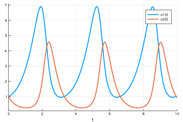
Next we define a single layer neural network that using the
AD-compatible concrete_solve function
function that takes the parameters and an initial condition and returns the
solution of the differential equation as a
DiffEqArray (same
array semantics as the standard differential equation solution object but without
the interpolations).
function predict_adjoint(p) # Our 1-layer neural network
  Array(concrete_solve(prob,Tsit5(),u0,p,saveat=0.0:0.1:10.0))
end
Next we choose a loss function. Our goal will be to find parameter that make
the Lotka-Volterra solution constant x(t)=1, so we defined our loss as the
squared distance from 1. Note that when using sciml_train, the first return
is the loss value, and the other returns are sent to the callback for monitoring
convergence.
function loss_adjoint(p)
  prediction = predict_adjoint(p)
  loss = sum(abs2,x-1 for x in prediction)
  loss,prediction
end
Lastly, we use the sciml_train function to train the parameters using BFGS to
arrive at parameters which optimize for our goal. sciml_train allows defining
a callback that will be called at each step of our training loop. It takes in the
current parameter vector and the returns of the last call to the loss function.
We will display the current loss and make a plot of the current situation:
cb = function (p,l,pred) #callback function to observe training
  display(l)
  # using `remake` to re-create our `prob` with current parameters `p`
  display(plot(solve(remake(prob,p=p),Tsit5(),saveat=0.0:0.1:10.0),ylim=(0,6)))
  return false # Tell it to not halt the optimization. If return true, then optimization stops
end

# Display the ODE with the initial parameter values.
cb(p,loss_adjoint(p)...)

res = DiffEqFlux.sciml_train(loss_adjoint, p, BFGS(initial_stepnorm = 0.0001), cb = cb)
* Status: failure (objective increased between iterations) (line search failed)
* Candidate solution
Minimizer: [1.44e+00, 1.44e+00, 2.54e+00, ...]
Minimum: 1.993849e-06
* Found with
Algorithm: BFGS
Initial Point: [1.50e+00, 1.00e+00, 3.00e+00, ...]
* Convergence measures
|x - x'| = 1.27e-09 ≰ 0.0e+00
|x - x'|/|x'| = 4.98e-10 ≰ 0.0e+00
|f(x) - f(x')| = 1.99e-12 ≰ 0.0e+00
|f(x) - f(x')|/|f(x')| = 1.00e-06 ≰ 0.0e+00
|g(x)| = 5.74e-03 ≰ 1.0e-08
* Work counters
Seconds run: 6 (vs limit Inf)
Iterations: 6
f(x) calls: 83
∇f(x) calls: 83In just seconds we found parameters which give a loss of 1e-6! We can get the
final loss with res.minimum, and get the optimal parameters with res.minimizer.
For example, we can plot the final outcome and show that we solved the control
problem and successfully found parameters to make the ODE solution constant:
plot(solve(remake(prob,p=res.minimizer),Tsit5(),saveat=0.0:0.1:10.0),ylim=(0,6))Here's an old video showing the use of the ADAM optimizer:
Other differential equation problem types from DifferentialEquations.jl are supported. For example, we can build a layer with a delay differential equation like:
function delay_lotka_volterra(du,u,h,p,t)
  x, y = u
  α, β, δ, γ = p
  du[1] = dx = (α - β*y)*h(p,t-0.1)[1]
  du[2] = dy = (δ*x - γ)*y
end
h(p,t) = ones(eltype(p),2)
u0 = [1.0,1.0]
prob = DDEProblem(delay_lotka_volterra,u0,h,(0.0,10.0),constant_lags=[0.1])

p = [2.2, 1.0, 2.0, 0.4]
function predict_dde(p)
  Array(concrete_solve(prob,MethodOfSteps(Tsit5()),u0,p,saveat=0.1,sensealg=TrackerAdjoint())
end
loss_dde(p) = sum(abs2,x-1 for x in predict_dde(p))
loss_dde(p)
Notice that we chose sensealg=TrackerAdjoint() to utilize the Tracker.jl
reverse-mode to handle the delay differential equation.
Or we can use a stochastic differential equation. Here we demonstrate
sensealg=ForwardDiffSensitivity() for forward-mode automatic differentiation
of a small stochastic differential equation:
function lotka_volterra_noise(du,u,p,t)
  du[1] = 0.1u[1]
  du[2] = 0.1u[2]
end
u0 = [1.0,1.0]
prob = SDEProblem(lotka_volterra,lotka_volterra_noise,u0,(0.0,10.0))

p = [2.2, 1.0, 2.0, 0.4]
function predict_sde(p)
  Array(concrete_solve(prob,SOSRI(),u0,p,sensealg=ForwardDiffSensitivity(),saveat=0.1))
end
loss_sde(p) = sum(abs2,x-1 for x in predict_sde(p))
loss_sde(p)
For this training process, because the loss function is stochastic, we will use
the ADAM optimizer from Flux.jl. The sciml_train function is the same as
before. However, to speed up the training process, we will use a global counter
so that way we only plot the current results every 10 iterations. This looks like:
iter = 0
cb = function (p,l)
  display(l)
  global iter
  if iter%10 == 0
      display(plot(solve(remake(prob,p=p),SOSRI(),saveat=0.1),ylim=(0,6)))
  end
  iter += 1
  return false
end

# Display the ODE with the current parameter values.
cb(p,loss_sde(p))

DiffEqFlux.sciml_train(loss_sde, p, ADAM(0.1), cb = cb, maxiters = 100)
We can use DiffEqFlux.jl to define, solve, and train neural ordinary differential
equations. A neural ODE is an ODE where a neural network defines its derivative
function. Thus for example, with the multilayer perceptron neural network
Chain(Dense(2,50,tanh),Dense(50,2)), the best way to define a neural ODE by hand
would be to use non-mutating adjoints, which looks like:
p,re = Flux.destructure(model)
dudt_(u,p,t) = re(p)(u)
prob = ODEProblem(dudt_,x,tspan,p)
my_neural_ode_prob = concrete_solve(prob,Tsit5(),u0,p,args...;kwargs...)(Flux.restructure and Flux.destructure are helper functions which transform
the neural network to use parameters p)
A convenience function which handles all of the details is NeuralODE. To
use NeuralODE, you give it the initial condition, the internal neural
network model to use, the timespan to solve on, and any ODE solver arguments.
For example, this neural ODE would be defined as:
tspan = (0.0f0,25.0f0)
n_ode = NeuralODE(model,tspan,Tsit5(),saveat=0.1)
where here we made it a layer that takes in the initial condition and spits out an array for the time series saved at every 0.1 time steps.
Let's get a time series array from the Lotka-Volterra equation as data:
using DiffEqFlux, OrdinaryDiffEq, Flux, Optim, Plots

u0 = Float32[2.; 0.]
datasize = 30
tspan = (0.0f0,1.5f0)

function trueODEfunc(du,u,p,t)
    true_A = [-0.1 2.0; -2.0 -0.1]
    du .= ((u.^3)'true_A)'
end
t = range(tspan[1],tspan[2],length=datasize)
prob = ODEProblem(trueODEfunc,u0,tspan)
ode_data = Array(solve(prob,Tsit5(),saveat=t))
Now let's define a neural network with a NeuralODE layer. First we define
the layer. Here we're going to use FastChain, which is a faster neural network
structure for NeuralODEs:
dudt2 = FastChain((x,p) -> x.^3,
            FastDense(2,50,tanh),
            FastDense(50,2))
n_ode = NeuralODE(dudt2,tspan,Tsit5(),saveat=t)
Note that we can directly use Chains from Flux.jl as well, for example:
dudt2 = Chain(x -> x.^3,
             Dense(2,50,tanh),
             Dense(50,2))
n_ode = NeuralODE(dudt2,tspan,Tsit5(),saveat=t)
In our model we used the x -> x.^3 assumption in the model. By incorporating structure
into our equations, we can reduce the required size and training time for the
neural network, but a good guess needs to be known!
From here we build a loss function around it. The NeuralODE has an optional
second argument for new parameters which we will use to iteratively change the
neural network in our training loop. We will use the L2 loss of the network's
output against the time series data:
function predict_n_ode(p)
  n_ode(u0,p)
end

function loss_n_ode(p)
    pred = predict_n_ode(p)
    loss = sum(abs2,ode_data .- pred)
    loss,pred
end

loss_n_ode(n_ode.p) # n_ode.p stores the initial parameters of the neural ODE
and then train the neural network to learn the ODE:
cb = function (p,l,pred;doplot=false) #callback function to observe training
  display(l)
  # plot current prediction against data
  if doplot
    pl = scatter(t,ode_data[1,:],label="data")
    scatter!(pl,t,pred[1,:],label="prediction")
    display(plot(pl))
  end
  return false
end

# Display the ODE with the initial parameter values.
cb(n_ode.p,loss_n_ode(n_ode.p)...)

res1 = DiffEqFlux.sciml_train(loss_n_ode, n_ode.p, ADAM(0.05), cb = cb, maxiters = 300)
cb(res1.minimizer,loss_n_ode(res1.minimizer)...;doplot=true)
res2 = DiffEqFlux.sciml_train(loss_n_ode, res1.minimizer, LBFGS(), cb = cb)
cb(res2.minimizer,loss_n_ode(res2.minimizer)...;doplot=true)

# result is res2 as an Optim.jl object
# res2.minimizer are the best parameters
# res2.minimum is the best loss
* Status: failure (reached maximum number of iterations)
* Candidate solution
Minimizer: [4.38e-01, -6.02e-01, 4.98e-01, ...]
Minimum: 8.691715e-02
* Found with
Algorithm: ADAM
Initial Point: [-3.02e-02, -5.40e-02, 2.78e-01, ...]
* Convergence measures
|x - x'| = NaN ≰ 0.0e+00
|x - x'|/|x'| = NaN ≰ 0.0e+00
|f(x) - f(x')| = NaN ≰ 0.0e+00
|f(x) - f(x')|/|f(x')| = NaN ≰ 0.0e+00
|g(x)| = NaN ≰ 0.0e+00
* Work counters
Seconds run: 5 (vs limit Inf)
Iterations: 300
f(x) calls: 300
∇f(x) calls: 300
* Status: success
* Candidate solution
Minimizer: [4.23e-01, -6.24e-01, 4.41e-01, ...]
Minimum: 1.429496e-02
* Found with
Algorithm: L-BFGS
Initial Point: [4.38e-01, -6.02e-01, 4.98e-01, ...]
* Convergence measures
|x - x'| = 1.46e-11 ≰ 0.0e+00
|x - x'|/|x'| = 1.26e-11 ≰ 0.0e+00
|f(x) - f(x')| = 0.00e+00 ≤ 0.0e+00
|f(x) - f(x')|/|f(x')| = 0.00e+00 ≤ 0.0e+00
|g(x)| = 4.28e-02 ≰ 1.0e-08
* Work counters
Seconds run: 4 (vs limit Inf)
Iterations: 35
f(x) calls: 336
∇f(x) calls: 336
Here we showcase starting the optimization with ADAM to more quickly find a
minimum, and then honing in on the minimum by using LBFGS. By using the two
together, we are able to fit the neural ODE in 9 seconds! (Note, the timing
commented out the plotting).
Note that the differential equation solvers will run on the GPU if the initial condition is a GPU array. Thus for example, we can define a neural ODE by hand that runs on the GPU:
u0 = Float32[2.; 0.] |> gpu
dudt = Chain(Dense(2,50,tanh),Dense(50,2)) |> gpu

p,re = DiffEqFlux.destructure(model)
dudt_(u,p,t) = re(p)(u)
prob = ODEProblem(ODEfunc, u0,tspan, p)

# Runs on a GPU
sol = solve(prob,Tsit5(),saveat=0.1)
and concrete_solve works similarly. Or we can directly use the neural ODE
layer function, like:
n_ode = NeuralODE(gpu(dudt2),tspan,Tsit5(),saveat=0.1)You can also mix a known differential equation and a neural differential equation, so that the parameters and the neural network are estimated simultaneously!
Here's an example of doing this with both reverse-mode autodifferentiation and with adjoints. We will assume that we know the dynamics of the second equation (linear dynamics), and our goal is to find a neural network that will control the second equation to stay close to 1.
using DiffEqFlux, Flux, Optim, OrdinaryDiffEq

u0 = Float32(1.1)
tspan = (0.0f0,25.0f0)

ann = FastChain(FastDense(2,16,tanh), FastDense(16,16,tanh), FastDense(16,1))
p1 = initial_params(ann)
p2 = Float32[0.5,-0.5]
p3 = [p1;p2]
θ = Float32[u0;p3]

function dudt_(du,u,p,t)
    x, y = u
    du[1] = ann(u,p[1:length(p1)])[1]
    du[2] = p[end-1]*y + p[end]*x
end
prob = ODEProblem(dudt_,u0,tspan,p3)
concrete_solve(prob,Tsit5(),[0f0,u0],p3,abstol=1e-8,reltol=1e-6)

function predict_adjoint(θ)
  Array(concrete_solve(prob,Tsit5(),[0f0,θ[1]],θ[2:end],saveat=0.0:1:25.0))
end
loss_adjoint(θ) = sum(abs2,predict_adjoint(θ)[2,:].-1)
l = loss_adjoint(θ)

cb = function (θ,l)
  println(l)
  #display(plot(solve(remake(prob,p=Flux.data(p3),u0=Flux.data(u0)),Tsit5(),saveat=0.1),ylim=(0,6)))
  return false
end

# Display the ODE with the current parameter values.
cb(θ,l)

loss1 = loss_adjoint(θ)
res = DiffEqFlux.sciml_train(loss_adjoint, θ, BFGS(initial_stepnorm=0.01), cb = cb)
* Status: success
* Candidate solution
Minimizer: [1.00e+00, 4.33e-02, 3.72e-01, ...]
Minimum: 6.572520e-13
* Found with
Algorithm: BFGS
Initial Point: [1.10e+00, 4.18e-02, 3.64e-01, ...]
* Convergence measures
|x - x'| = 0.00e+00 ≤ 0.0e+00
|x - x'|/|x'| = 0.00e+00 ≤ 0.0e+00
|f(x) - f(x')| = 0.00e+00 ≤ 0.0e+00
|f(x) - f(x')|/|f(x')| = 0.00e+00 ≤ 0.0e+00
|g(x)| = 5.45e-06 ≰ 1.0e-08
* Work counters
Seconds run: 8 (vs limit Inf)
Iterations: 23
f(x) calls: 172
∇f(x) calls: 172Notice that in just 23 iterations or 8 seconds we get to a minimum of 7e-13,
successfully solving the nonlinear optimal control problem.
With neural stochastic differential equations, there is once again a helper form neural_dmsde which can
be used for the multiplicative noise case (consult the layers API documentation, or
this full example using the layer function).
However, since there are far too many possible combinations for the API to
support, in many cases you will want to performantly define neural differential
equations for non-ODE systems from scratch. For these systems, it is generally
best to use TrackerAdjoint with non-mutating (out-of-place) forms. For example,
the following defines a neural SDE with neural networks for both the drift and
diffusion terms:
dudt_(u,p,t) = model(u)
g(u,p,t) = model2(u)
prob = SDEProblem(dudt_,g,x,tspan,nothing)
where model and model2 are different neural networks. The same can apply to a neural delay differential equation.
Its out-of-place formulation is f(u,h,p,t). Thus for example, if we want to define a neural delay differential equation
which uses the history value at p.tau in the past, we can define:
dudt_(u,h,p,t) = model([u;h(t-p.tau)])
prob = DDEProblem(dudt_,u0,h,tspan,nothing)First let's build training data from the same example as the neural ODE:
using Flux, DiffEqFlux, StochasticDiffEq, Plots, DiffEqBase.EnsembleAnalysis, Statistics

u0 = Float32[2.; 0.]
datasize = 30
tspan = (0.0f0,1.0f0)

function trueSDEfunc(du,u,p,t)
    true_A = [-0.1 2.0; -2.0 -0.1]
    du .= ((u.^3)'true_A)'
end
t = range(tspan[1],tspan[2],length=datasize)
mp = Float32[0.2,0.2]
function true_noise_func(du,u,p,t)
    du .= mp.*u
end
prob = SDEProblem(trueSDEfunc,true_noise_func,u0,tspan)
For our dataset we will use DifferentialEquations.jl's parallel ensemble interface to generate data from the average of 10000 runs of the SDE:
# Take a typical sample from the mean
ensemble_prob = EnsembleProblem(prob)
ensemble_sol = solve(ensemble_prob,SOSRI(),trajectories = 10000)
ensemble_sum = EnsembleSummary(ensemble_sol)
sde_data,sde_data_vars = Array.(timeseries_point_meanvar(ensemble_sol,t))
Now we build a neural SDE. For simplicity we will use the NeuralDSDE
neural SDE with diagonal noise layer function:
drift_dudt = FastChain((x,p) -> x.^3,
             FastDense(2,50,tanh),
             FastDense(50,2))
diffusion_dudt = FastChain(FastDense(2,2))
n_sde = NeuralDSDE(drift_dudt,diffusion_dudt,tspan,SOSRI(),saveat=t,reltol=1e-1,abstol=1e-1)
Let's see what that looks like:
pred = n_sde(u0) # Get the prediction using the correct initial condition
drift_(u,p,t) = drift_dudt(u,p[1:n_sde.len])
diffusion_(u,p,t) = diffusion_dudt(u,p[(n_sde.len+1):end])
nprob = SDEProblem(drift_,diffusion_,u0,(0.0f0,1.2f0),n_sde.p)

ensemble_nprob = EnsembleProblem(nprob)
ensemble_nsol = solve(ensemble_nprob,SOSRI(),trajectories = 100, saveat = t)
ensemble_nsum = EnsembleSummary(ensemble_nsol)
p1 = plot(ensemble_nsum, title = "Neural SDE: Before Training")
scatter!(p1,t,sde_data',lw=3)
scatter(t,sde_data[1,:],label="data")
scatter!(t,pred[1,:],label="prediction")
Now just as with the neural ODE we define a loss function that calculates the
mean and variance from n runs at each time point and uses the distance
from the data values:
function predict_n_sde(p)
  Array(n_sde(u0,p))
end
function loss_n_sde(p;n=100)
  samples = [predict_n_sde(p) for i in 1:n]
  means = reshape(mean.([[samples[i][j] for i in 1:length(samples)] for j in 1:length(samples[1])]),size(samples[1])...)
  vars = reshape(var.([[samples[i][j] for i in 1:length(samples)] for j in 1:length(samples[1])]),size(samples[1])...)
  loss = sum(abs2,sde_data - means) + sum(abs2,sde_data_vars - vars)
  loss,means,vars
end

cb = function (p,loss,means,vars) #callback function to observe training
  # loss against current data
  display(loss)
  # plot current prediction against data
  pl = scatter(t,sde_data[1,:],yerror = sde_data_vars[1,:],label="data")
  scatter!(pl,t,means[1,:],ribbon = vars[1,:], label="prediction")
  display(plot(pl))
  return false
end

# Display the SDE with the initial parameter values.
cb(n_sde.p,loss_n_sde(n_sde.p)...)
Now we train using this loss function. We can pre-train a little bit using
a smaller n and then decrease it after it has had some time to adjust towards
the right mean behavior:
opt = ADAM(0.025)
res1 = DiffEqFlux.sciml_train((p)->loss_n_sde(p,n=10),  n_sde.p, opt, cb = cb, maxiters = 100)
res2 = DiffEqFlux.sciml_train((p)->loss_n_sde(p,n=100), res1.minimizer, opt, cb = cb, maxiters = 100)
And now we plot the solution to an ensemble of the trained neural SDE:
samples = [predict_n_sde(res2.minimizer) for i in 1:1000]
means = reshape(mean.([[samples[i][j] for i in 1:length(samples)] for j in 1:length(samples[1])]),size(samples[1])...)
vars = reshape(var.([[samples[i][j] for i in 1:length(samples)] for j in 1:length(samples[1])]),size(samples[1])...)

p2 = scatter(t,sde_data',yerror = sde_data_vars',label="data", title = "Neural SDE: After Training", xlabel="Time")
plot!(p2,t,means',lw = 8,ribbon = vars', label="prediction")

plot(p1,p2,layout=(2,1))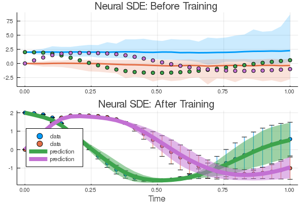
Try this with GPUs as well!
As shown in the stiff ODE tutorial, differential-algebraic equations
(DAEs) can be used to impose physical constraints. One way to define a DAE is
through an ODE with a singular mass matrix. For example, if we make Mu = f(u)
where the last row of M is all zeros, then we have a constraint defined by
the right hand side. Using NeuralODEMM, we can use this to define a neural
ODE where the sum of all 3 terms must add to one. An example of this is as
follows:
using Flux, DiffEqFlux, OrdinaryDiffEq, Optim, Test
#A desired MWE for now, not a test yet.
function f(du,u,p,t)
    y₁,y₂,y₃ = u
    k₁,k₂,k₃ = p
    du[1] = -k₁*y₁ + k₃*y₂*y₃
    du[2] =  k₁*y₁ - k₃*y₂*y₃ - k₂*y₂^2
    du[3] =  y₁ + y₂ + y₃ - 1
    nothing
end
u₀ = [1.0, 0, 0]
M = [1. 0  0
     0  1. 0
     0  0  0]
tspan = (0.0,1.0)
p = [0.04,3e7,1e4]
func = ODEFunction(f,mass_matrix=M)
prob = ODEProblem(func,u₀,tspan,p)
sol = solve(prob,Rodas5(),saveat=0.1)

dudt2 = FastChain(FastDense(3,64,tanh),FastDense(64,2))
ndae = NeuralODEMM(dudt2, (u,p,t) -> [u[1] + u[2] + u[3] - 1], tspan, M, Rodas5(autodiff=false),saveat=0.1)
ndae(u₀)

function predict_n_dae(p)
    ndae(u₀,p)
end
function loss(p)
    pred = predict_n_dae(p)
    loss = sum(abs2,sol .- pred)
    loss,pred
end

cb = function (p,l,pred) #callback function to observe training
  display(l)
  return false
end

l1 = first(loss(ndae.p))
res = DiffEqFlux.sciml_train(loss, ndae.p, BFGS(initial_stepnorm = 0.001),
                             cb = cb, maxiters = 100)
@test res.minimum < l1
This is a highly stiff problem, making the fitting difficult, but we have manually
imposed that sum constraint via (u,p,t) -> [u[1] + u[2] + u[3] - 1], making
the fitting easier.
For the sake of not having a never-ending documentation of every single combination of CPU/GPU with every layer and every neural differential equation, we will end here. But you may want to consult this blog post which showcases defining neural jump diffusions and neural partial differential equations.
NeuralODE(model,tspan,solver,args...;kwargs...)defines a neural ODE layer wheremodelis a Flux.jl model,tspanis the time span to integrate, and the rest of the arguments are passed to the ODE solver.NeuralODEMM(model,constraints,tspan,mass_matrix,args...;kwargs...)defines a neural ODE layer with a mass matrix, i.e.Mu=[model(u);constraints(u,p,t)]where the constraints cover the rank-deficient area of the mass matrix (i.e., the constraints of a differential-algebraic equation). Thus the mass matrix is allowed to be singular.NeuralDSDE(model1,model2,tspan,solver,args...;kwargs...)defines a neural SDE layer wheremodel1is a Flux.jl for the drift equation,model2is a Flux.jl model for the diffusion equation,tspanis the time span to integrate, and the rest of the arguments are passed to the SDE solver. The noise is diagonal, i.e. it assumes a vector output and performsmodel2(u) .* dWagainst a dW matching the number of states.NeuralSDE(model1,model2,tspan,nbrown,solver,args...;kwargs...)defines a neural SDE layer wheremodel1is a Flux.jl for the drift equation,model2is a Flux.jl model for the diffusion equation,tspanis the time span to integrate,nbrownis the number of Brownian motions, and the rest of the arguments are passed to the SDE solver. The model is multiplicative, i.e. it's interpreted asmodel2(u) * dW, and so the return ofmodel2should be an appropriate matrix for performing this multiplication, i.e. the size of its output should belength(x) x nbrown.NeuralCDDE(model,tspan,lags,solver,args...;kwargs...)defines a neural DDE layer wheremodelis a Flux.jl model,tspanis the time span to integrate, lags is the lagged values to use in the predictor, and the rest of the arguments are passed to the ODE solver. The model should take in a vector that concatenates the lagged states, i.e.[u(t);u(t-lags[1]);...;u(t-lags[end])]
A raw ODE solver benchmark showcases a 50,000x performance advantage over torchdiffeq on small ODEs.