AdamSturge/geometry-processing-curvature

Curvature assignment for Geometry Processing course

Geometry Processing – Curvature

To get started: Fork this repository then issue

git clone --recursive http://github.com/[username]/geometry-processing-curvature.git

Installation, Layout, and Compilation

See introduction.

Execution

Once built, you can execute the assignment from inside the build/ by running on a given mesh:

./curvature [path to mesh.obj]

Background

In this assignment we explore discrete curvature quantities computed on a surface. These quantities give us local information about a shape. Beyond inspecting the surface (the extent of this assignment), these quantities become the building blocks to:

• define energies to minimize during smoothing/deformation,
• identify salient points and curves on the shape, and
• provide initial conditions/constraints for remeshing.

The fundamental difference between a segment on the real line and a curve is the introduction of curvature. This is quite natural and intuitive. When we draw a 1D object in the plane or in space we have the freedom to let that object bend. We quantify this "bending" locally as curvature.

Curvature is also the fundamental difference between a chunk (i.e., subregion) of the Euclidean Plane and a surface that has been immersed in $\R^3$ (or elsewhere). Unlike curves, surfaces can bend in each direction at any point.

We start our discussion assuming a smooth surface $\S$. We would like to categorize points on the surface $\p ∈ \S$ in terms of how the surface bends or curves locally.

Curvature of planar curves

Let us briefly recall how curvature is defined for a planar curve $γ:[0,1] → \R²$.

There are multiple equivalent definitions.

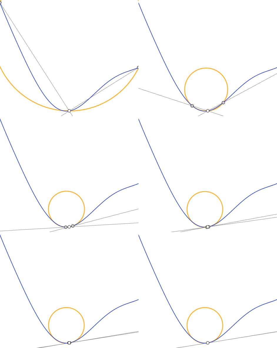
Osculating circle

We can define the tangent direction at a point $\p = γ(s)$ as the limit of the secant formed between $\p$ and another point on the curve $\q = γ(t)$ as $\q$ approaches $\p$:

\[ \t(s) = \lim_{\q→\p} \frac{\q-\p}{|\q-\p|} = \lim_{t→s} \frac{γ(t)-γ(s)}{|γ(t)-γ(s)|} = \frac{γ'(s)}{|γ'(s)|}. \] It always possible, and often convenient, to assume without loss of generality that $s$ is an arc length parameterization of the curve $γ$ so that $|γ'| = 1$ and therefor the unit tangent vector is simply $\t(s) = γ'(s)$.

In an analogous fashion, we can consider the limit of the circumcircle $C(\q₁,\p,\q₂)$ that passes through $\p$ and points $\q₁$ and $\q₂$ before and after it on the curve:

\[ C(\p) = \lim_{\q₁,\q₂→\p} C(\q₁,\p,\q₂). \]

This limit circle is called the osculating circle at the point $\p$ on the curve $γ$. By construction the tangent of the curve and the circle match at $\p$: they're both $γ'$. The radius $R(\p)$ of the osculating circle $C(\p)$ at the the point $\p$ is proportional to how straight the curve is locally: as the curve becomes more and more straight then the radius tends toward infinity. This implies that the radius is inversely proportional to the "curvy-ness" of the curve. Hence, the inverse of the radius is dubbed the curvature:

\[ κ(\p) = \frac{1}{R(\p)}. \] The radius is a non-negative measure of length with units meters, so the curvature $κ$ is an non-negative scalar with units 1/meters. The radius of the osculating circle can also be written as a limit of the circumcircle radius:

\[ R(\p) = \lim_{\q₁,\q₂→\p} \frac{‖\q₁-\p‖ ‖\p-\q₂‖ ‖\q₂-\q₁‖} {2\left| (\q₁-\p) \quad (\p-\q₂)\right|}. \]

Signed curvature

Plugging in our arc-length parameterization this reveals that the curvature (inverse of radius) is equal to the magnitude of change in the tangent or equivalently the magnitude of second derivative of the curve:

\[ κ(s) = \lim_{t→s} \left| \frac{γ'(t)-γ'(s)}{t-s} \right| = ‖γ''(s)‖. \]

Because we chose the arc-length parameterization, the only change to the tangent vector $γ'$ is a change in direction (as opposed to magnitude, since $‖γ'‖ := 1$). This means that the change--as a vector itself--is orthogonal to the tangent. In other words, the change in tangent $γ''$ points along the normal direction $\hat{\n}$:

\[ γ'' ⋅ γ' = 0 \quad → \quad γ'' ⋅ \hat{\n} = ± κ \hat{\n}. \label{equ:curvature-normal} \]

If we define an orientation to our curve then we can endow the curvature with a sign based on whether the center of the osculating circle lies on the left or right side of the curve. As already established, the tangent of the osculating circle and the curve agree, so the vector pointing toward the circle's center must be perpendicular to the tangent: i.e., in either the positive or negative normal directions.

If the orientation agrees with increasing the arc-length parameter $s$, then the sign can be determined by comparing the second derivative vector $γ''$ to the unit normal $\hat{\n} := (γ')^⊥$. The signed curvature at a point $\p$ is thus given by:

\[ \begin{align} k(\p) &= \text{sign}(γ''(\p)⋅\hat{\n}))\ κ(\p) \ &= γ''(\p) ⋅ \hat{\n}. \end{align} \]

Moving point analogy

This definition neatly conforms to our intuition of a curve as the trajectory of a moving point. Imagine the curved formed by driving along a particular trajectory $γ(t)$, where we really interpret $t$ as time.

While $γ'(t)$ corresponds to your velocity vector and $‖γ'(t)‖$ corresponds to your speed, the arc-length (re-)parameterization would correspond to having your friend re-trace your path traveling at a perfectly uniform speed $‖γ'(s)‖ = 1$, where your friends "time" $s$ may be different from yours (it may take longer or shorter depending if you drove fast or slow).

Curvature in the path corresponds to turning and quite literally the amount by which your friend needs to turn the steering wheel away from the "straight" position: on a straight course, the steering wheel remains at zero-angle position and the curvature is zero, on a circular course the steering wheel is fixed at a constant angle in the left or right direction corresponding to constant positive or negative curvature respectively.

Changing the steering wheel changes the direction of the vehicle's velocity. For your friend driving at constant speed, this is the only change admissible to the velocity, hence the curvature exactly corresponds to $γ''(s)$ and to the steering wheel angle.

If somebody wants to make a Sega Out Run inspired gif showing a steering wheel turning next to a little car tracing a curve, I'll be very impressed.

Turning number

The integrated signed curvature around a closed curve must be an integer multiple of $2π$:

\[ ∮ k(s) \ ds = 2π τ, \] where τ is an integer called the "turning number" of the curve.

This is a bit surprising at first glance. However, in the moving point analogy a closed curve corresponds to a period trajectory (e.g., driving around a race-track). When we've made it once around the track, our velocity direction (e.g., the direction the vehicle is facing) must be pointing in the original direction. That is, during the course, the car either have turned all the way around once ($τ = 1$) or turned as much clockwise and it did counter-clockwise (e.g., on a figure 8 course: $τ=0$), or made multiple loops, etc.

Discrete curvature

In the discrete world, if a curve is represented as a piecewise-linear chain of segments, then it's natural to associate curvature with vertices: the segments are flat and therefor contain no curvature.

A natural analog to the definition of curvature as the derivative of the tangent vector (i.e., $k = ‖γ''‖ = ‖\t'‖$) is to define discrete curvature as the change in tangent direction between discrete segments meeting at a vertex:

\[ k_i = ∠ (\v_i - (\v_{i-1}-\v_i)) \v_i\v_{i+1} = θ_i, \] that is, the signed exterior angle $θ_i$ at the vertex $\v_i$.

The turning number theorem for continuous curves finds an immediate analog in the discrete case. For a closed polygon the discrete signed angles must sum up to a multiple of $2π$ in order to close up:

\[ ∑_{i=1}^n k_i = 2π τ. \]

In this way, we preserve the structure found in the continuous case in our discrete analog. This structure preservation leads to an understanding of the exterior angle as an approximation or discrete analog of the locally integrated curvature.

Alternatively, we could literally fit an circle to the discrete curve based on local samples and approximate curvature as the inverse radius of the osculating circle. This curvature measure (in general) will not obey the turning number theorem, but (conducted properly) it will converge to the pointwise continuous values under refinement (e.g., as segment length shrinks).

We will explore these two concepts for surfaces, too: discrete analogs that preserve continuous structures and discretizations that approximate continuous quantities in the limit.

Curvature(s) on surfaces

A surface can be curved locally in multiple ways. Consider the difference between a flat piece of paper, a spherical ping-pong ball and a saddle-shaped Pringles chip. The Pringles chip is the most interesting because it curves "outward" in one direction and "inward" in another direction. In this section, we will learn to distinguish and classify points on a surface based on how it curves in each direction.

Normal curvature

The simplest way to extend the curvature that we defined for planar curves to a surface $\S$ is to slice the surface through a given point $\p∈\S$ with a plane $\P$ that is parallel to the surface normal $\n(\p)$.

The (local) intersection of the surface $\S$ and the plane $\P$ will trace a curve $γ$, upon which we can immediately use the planar curvature definition above.

There are infinitely many planes that pass through a given point $\p$ and lie parallel to a given normal vector $\n(\p)$: the plane can rotate around the normal $\n(\p)$ by any angle $φ$. For each choice of $φ$, the plane will define an intersecting curve $γ_φ$ and thus for every angle $φ$ there will be a normal curvature:

\[ k_\n(φ,\p) = γ''_\n(\p). \]

Mean curvature

Normal curvature requires choosing an angle, so it doesn't satiate our desire to reduce the "curvy-ness" to a single number for any point on the surface. A simple way to reduce this space of normal curvatures is to, well, average all possible normal curvatures. This defines the mean curvature:

\[ H(\p) = \frac{1}{2π}∫_0^{2π} k_\n(φ,\p) \ dφ. \]

Maximum and minimum curvature

Another obvious way to reduce the space of normal curvatures to a single number is to consider the maximum or minimum normal curvature over all choices of $φ$:

\[ \begin{align} k₁(\p) &= \max_φ \ k_\n(φ,\p) \ k₂(\p) &= \min_φ \ k_\n(φ,\p). \end{align} \]

Collectively, these are referred to as the principal curvatures and correspondingly the angles that maximize and minimize curvature are referred to as the principle curvature directions:

\[ \begin{align} φ₁(\p) &= \argmax_φ \ k_\n(φ,\p) \ φ₂(\p) &= \argmin_φ \ k_\n(φ,\p). \end{align} \]

Euler's theorem states that the normal curvature is a quite simple function of $φ$ and the principle curvatures:

\[ k_\n(φ,\p) = k₁ \cos^2 φ + k₂ \sin^2 φ. \]

There are two immediate and important consequences:

1. the principal curvature directions ($φ₁$ and $φ₂$) are orthogonal, and
2. the mean curvature reduces to the average of principal curvatures:

\[ H = ½(k₁ + k₂). \]

For more theory and a proof of Euler's theorem, I recommend "Elementary Differential Geometry" by Barret O'Neill, Chapter 5.2.

Gaussian curvature

Maximum, minimum and mean curvature reduce curvature to a single number, but still cannot (alone) distinguish between points lying on a round ping-pong ball, a flat sheet of paper, the cylindrical Pringles can and a saddle-shaped Pringles chip.

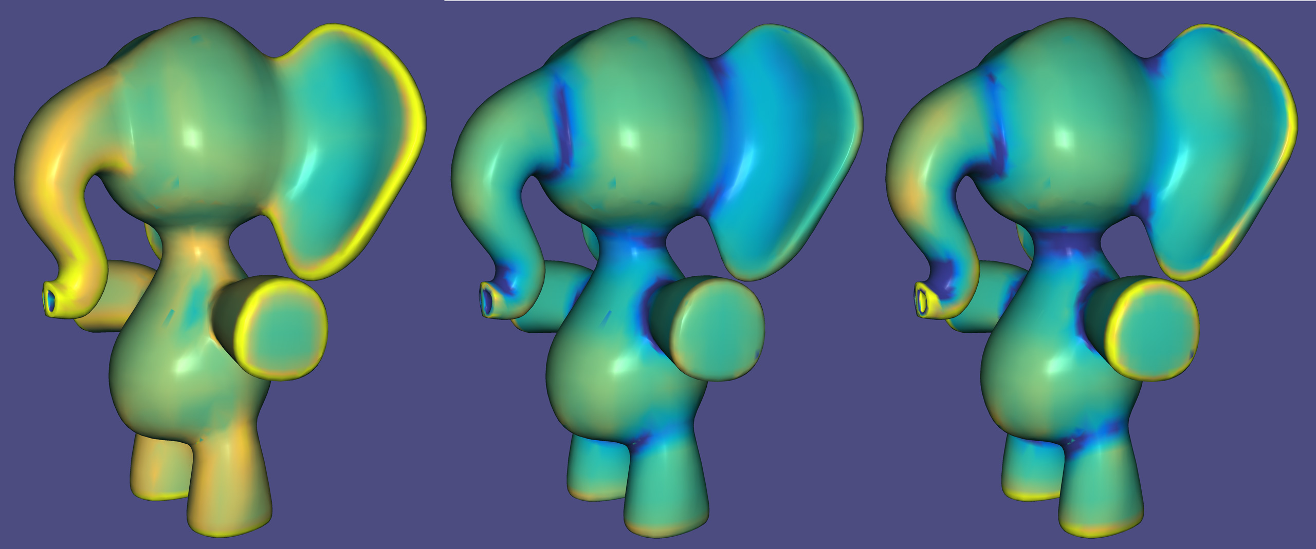
The neck of this cartoon elephant--like a Pringles chip--bends inward in one direction (positive $k₁ > 0$) and outward in the other direction (negative $k₂ < 0$).

The product of the principal curvatures maintains the disagreement in sign that categories this saddle-like behavior. This product is called Gaussian curvature:

\[ K = k_1 k_2. \]

Relationship to surface area

Both mean and Gaussian curvature have meaningful relationships to surface area.

Mean Curvature as area gradient

Let us consider a seemingly unrelated yet familiar problem. Suppose we would like to minimize the surface area of a given shape $\S$.

If we consider a small patch $A ⊂ \S$ centered around some point $\p ∈\S$, then we can imagine forces at the boundary of the patch $∂A$ that try to shrink the area of the patch. These "surface tension" forces point inward against the normal direction of the patch boundary $η$. Consider the integral effect of these forces and apply divergence theorem to move the integral to the interior of the patch.

\[ ∮_{∂A} -η ;ds = ∮_{∂A} \n × d\x = ∫_A ∆\x ;dA, \] where $\n$ is the surface normal, $d\x$ is the infinitesimal change in position around the boundary of the patch, and $∆\x ∈ \R³$ computes the Laplacian of the position coordinate functions.

In the limit as $A$ shrinks around any point on the surface, this relationship gives us the intuition that moving the surface in the direction $∆\x$ will decrease the surface area.

The Laplacian $∆f$ of a function $f$ on the surface does not depend on the choice of parameterization. It is defined as the divergence of the gradient of the function or equivalently the trace of the Hessian:

\[ ∆f = ∇⋅ ∇f = \tr{ \left[ \begin{array}{cc} \frac{∂²f}{∂u²} & \frac{∂²f}{∂u∂v} \ \frac{∂²f}{∂v∂u} & \frac{∂²f}{∂v²} \end{array} \right] }

\frac{∂²f}{∂u²} + \frac{∂²f}{∂v²}. \]

If we generously choose $u$ and $v$ to vary in the principal directions $φ₁$ and $φ₂$ above. In this case, the Laplacian $∆\x$ of the position function reduces to the sum of principal curvatures times the normal (recall Equation $(\ref{equ:curvature-normal})$):

\[ \begin{align} ∆\x &= \frac{∂²\x}{∂u²} + \frac{∂²\x}{∂v²} \ &= k₁ \n + k₂ \n \ &= 2H\n, \end{align} \] where $H\n ∈ \R³$ is called the mean curvature normal vector. We have shown that the mean curvature normal is equal half the Laplacian of the embedding function.

Gaussian Curvature as area distortion

As the product of principal curvatures, Gaussian curvature $K = k₁k₂$ measures zero anytime one (or both) of the principal curvatures are zero. Intuitively, this happens only for surfaces that curve or bend in one direction. Imagine rolling up a sheet of paper. Surfaces with zero Gaussian curvature $K = 0$ are called developable surfaces because the can be flattened (developed) on to the flat plane (just as you might unroll the piece of paper) without stretching or shearing. As a corollary, surfaces with non-zero Gaussian curvature cannot be flattened to the plane without stretching some part.

Locally, Gaussian curvature measures how far from developable the surface is: how much would the local area need to stretch to become flat.

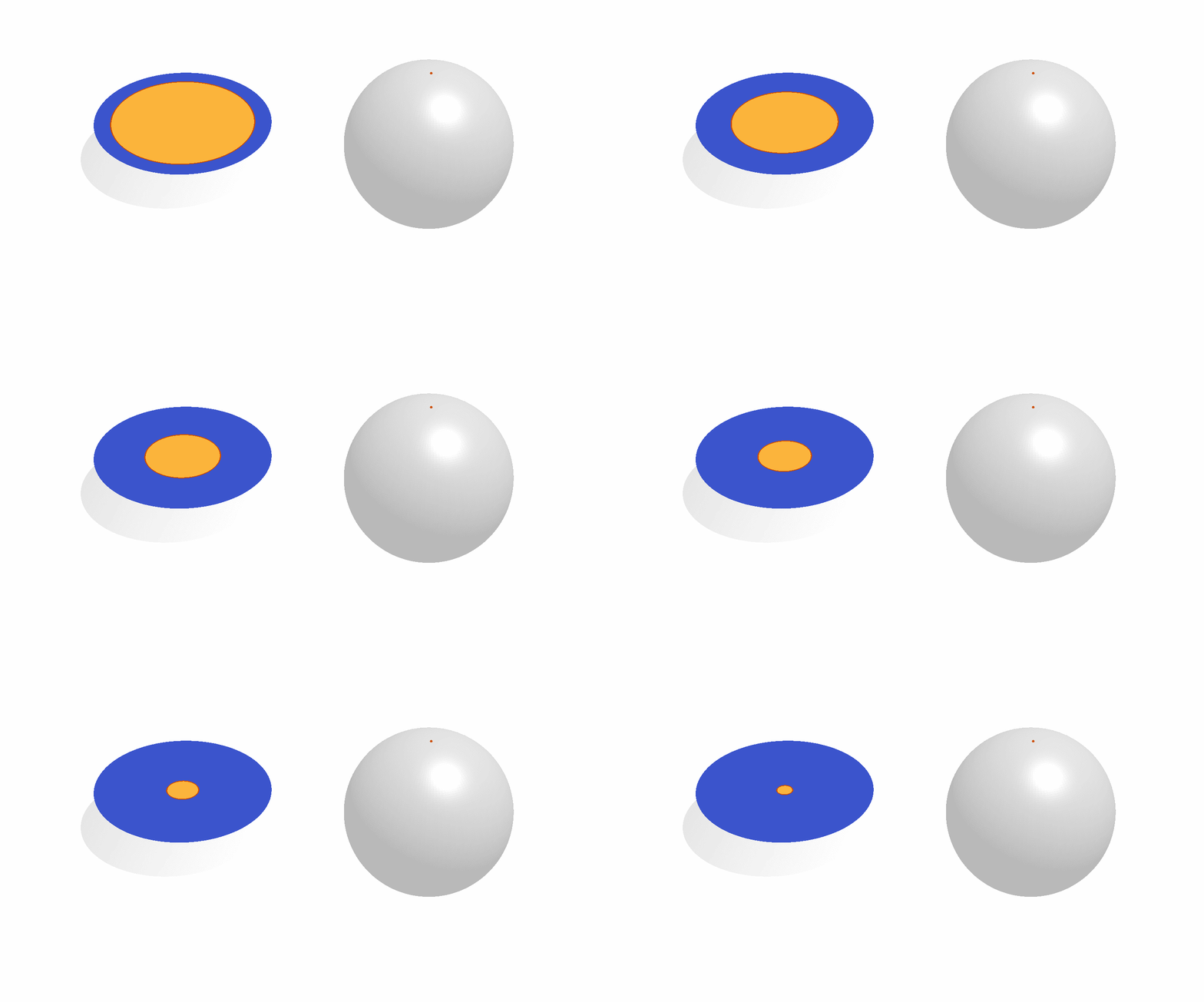
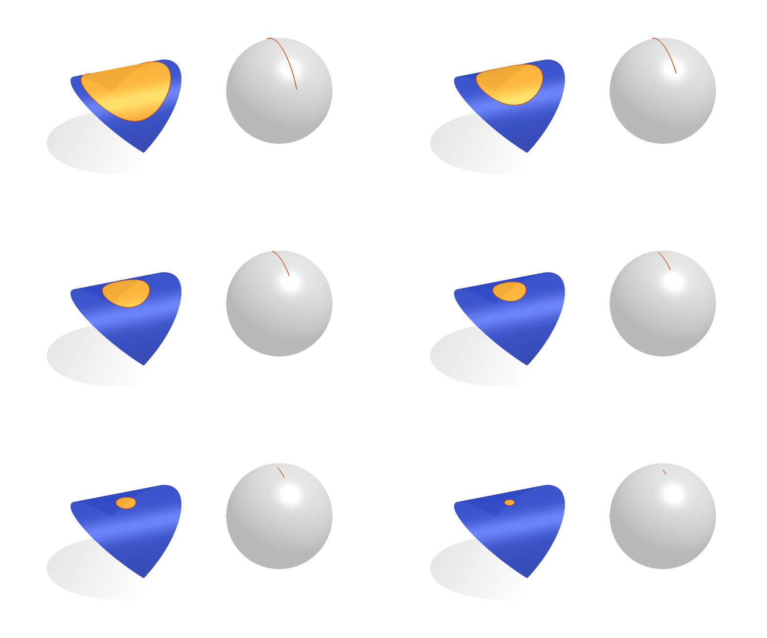
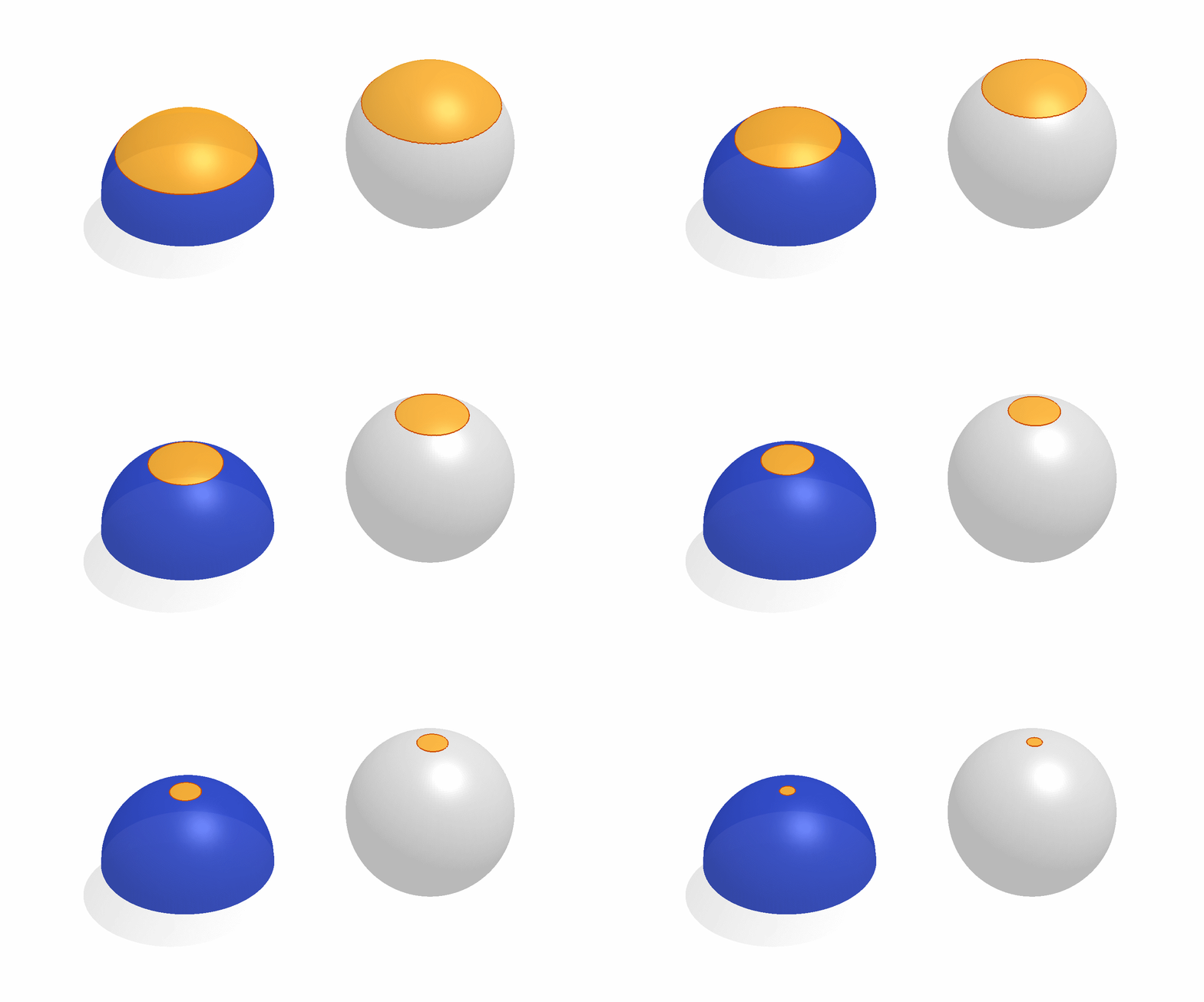
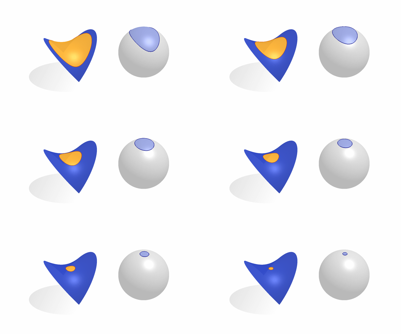
First, we introduce the Gauss map, a continuous map $N:\S→S²$ from every point $\p$ on the surface $\S$ to the unit sphere $S²$ so that $N(\p) := \n(\p)$, the unit normal at $\p$.

Consider a small patch on a curved surface. Gaussian curvature $K$ can equivalently be defined as the limit of the ratio between the area area swept out by the unit normal on the Gauss map $A_G$ and the area of the surface patch $A$:

\[ K = \lim_{A→0} \frac{A_G}{A}. \label{equ:gaussian-curvature-area} \]

Let's consider different types of regions:

• flat: $A_G=0$ because the Gauss map is a point,
• cylindrical: $A_G=0$ because the Gauss map is a curve,
• spherical: $A_G>0$ because the Gauss map will maintain positive swept-area, and
• saddle-shaped: $A_G<0$ because the area on the Gauss map will maintain oppositely oriented area (i.e., from the spherical case).

Similar to the turning number theorem for curves, there exists an analogous theorem for surfaces stating that the total Gaussian curvature must be an integer multiple of $2π$:

\[ ∫_S K dA = 2π χ(\S), \label{equ:gauss-bonnet} \] where $χ(\S)$ is the Euler characteristic of the surfaces $\S$ (a topological invariant of the surface revealing how many holes the surface has).

In stark contrast to mean curvature, this theorem tells us that we cannot add Gaussian curvature to a surface without:

1. removing an equal amount some place else, or
2. changing the topology of the surface.

Since changing the topology of the surface would require a discontinuous deformation, adding and removing Gaussian curvature must also balance out for smooth deformations. This simultaneously explains why a cloth must have wrinkles when draping over a table, and why a deflated basketball will not lie flat on the ground.

Shape operator

There is yet another way to arrive at principal, mean and Gaussian curvatures. Consider a point $\p$ on a surface $\S$ with unit normal vector $\n$. If we pick a unit tangent vector $\v$ (i.e., so that $\v ⋅ \n = 0$), then we can ask how does the normal $\n$ change as we move in the direction of $\v$ along the surface:

\[ S_\p(\v) := ∇ \n ⋅ \v \] we call $S_\p$ the shape operator at the point $\p$. Just as how in Equation $(\ref{equ:curvature-normal})$ the curvature normal must point in the normal direction, the shape operator takes as input a tangent vector and outputs another tangent vector (i.e., the change in the unit normal must be tangential to the surface; no change can occur in the normal direction itself).

Locally, the tangent vector space is two-dimensional spanned by basis vectors $\e₁,\e₂ ∈ \R²$ so we can think of the shape operator as a mapping from $\R²$ to $\R²$. As a differential operator, the shape operator is a linear operator. This means we can represent its action on a tangent vector $\v = x₁ \e₁ + x₂\e₂$ as a matrix:

\[ S_\p(\v) = \left[ \begin{array}{cc} S_\p(\e₁)⋅\e₁ & S_\p(\e₁)⋅\e₂ \ S_\p(\e₂)⋅\e₁ & S_\p(\e₂)⋅\e₂ \end{array} \right] \v \]

Given $\r₁$ and $\r₂$ are the principal curvature directions (as unit 2D tangent vectors) we can rotate our coordinate frame to align $\e₁$ and $\e₂$ with the principal curvature directions. The shape operator takes on a very special form:

\[ S_\p = \left[\r₁ \quad \r₂\right] \left[ \begin{array}{cc} k₁ & 0 \ 0 & k² \end{array} \right] \left[\r₁ \quad \r₂\right]^\transpose \]

Consider why the off-diagonal terms are zero. Think about the extremality of the principal curvatures.

We have actually conducted an eigen decomposition on the shape operator. Reading this progression backwards, the eigen decomposition of the shape operator expressed in any basis will reveal:

1. the principal curvatures as the eigen values, and
2. the principal curvature directions as the eigen vectors.

Discrete curvatures on surfaces

Discrete mean curvature normal via discrete Laplace

By now we are very familiar with the discrete Laplacian for triangle meshes:

\[ ∆f ≈ \M^{-1} \L \f, \] where $\M,\L ∈\R^{n×n}$ are the mass and cotangent matrices respectively.

When applied to the vertex positions, this operator gives a point-wise (or rather integral average) approximation of the mean curvature normal:

\[ H\n ≈ \H = \M^{-1} \L \V ∈ \R^{n×3}. \]

Stripping the magnitude off the rows of the resulting matrix would give the unsigned mean curvature. To make sure that the sign is preserved we can check whether each row in $\H$ agrees or disagrees with consistently oriented per-vertex normals in $\N ∈ \R^{n×3}$.

This connection between the Laplace operator and the mean curvature normal provides additional understanding for its use as a geometric smoothing operator (see "Computing Discrete Minimal Surfaces and Their Conjugates" [Pinkall and Polthier 1993]).

Discrete Gaussian curvature via angle defect

On a discrete surface represented as a triangle mesh, curvature certainly can't live on the flat faces. Moreover, Gaussian curvature can't live along edges because we can always develop the triangles on either side of an edge to the plane without stretching them. In fact we can develop any arbitrarily long chain of faces connected by edges so long as it doesn't form a loop or contain all faces incident on a vertex. This hints that discrete Gaussian curvature (like curvature for curves) must live at vertices.

Using the definition of Gaussian curvature in terms of the area on the Gauss map in Equation $(\ref{equ:gaussian-curvature-area})$: flat faces correspond points on the Gauss map (contributing nothing), edges correspond to area-less curves (traced by their dihedral angles), but vertices correspond to spherical polygons connecting face normal-points. The area $Ω$ subtended on the Gauss map is call the solid angle. Conveniently, this area is simply the angle defect of internal angles $θ_f$ incident on the $i$-th vertex contributed by each $f$-th incident face:

\[ Ω_i = 2π - ∑\limits_{f ∈ \text{faces(i)}} θ_{if}. \]

Thus, our discrete analog of locally integrated Gaussian curvature is given as the angle defect at the $i$-th vertex. The local integral average (or pointwise) discrete Gaussian curvature is the angle defect divided by the local area associated with the $i$-th vertex:

\[ K_i = \frac{2π - ∑\limits_{f ∈ \text{faces(i)}} θ_{if}}{A_i}. \]

By way of closing up the Gauss map, closed polyhedral surfaces (i.e., meshes) will obey the Gauss-Bonnet in Equation $(\ref{equ:gauss-bonnet})$, too:

\[ ∑\limits_{i=1}^n K_i = 2π χ(\S). \]

We can connect this to Euler's formula for polyhedra in our very first assignment:

\[ \frac{1}{2π} ∑\limits_{i=1}^n K_i = |V| - |E| + |F|, \] where $|V|, |E|, |F|$ are the number of vertices, edges and faces respectively.

Approximation and eigen decomposition of the shape operator

Alternatively, we can approximate all curvatures of a surface by locally fitting an analytic surface and reading off its curvature values. Since planes have no curvature, the simplest type of analytic surface that will give a non-trivial curvature value is a quadratic surface.

Thus, the algorithm proceeds as follows. For each vertex $\v$ of the given mesh,

1. gather a sampling of points in the vicinity. For simplicity, let's just grab all other vertices that share an edge with $\v$ or share an edge with a vertex that shares an edge with $\v$ (i.e., the "two-ring" of $\v$). For most sane meshes, this will provide enough points. Gather the positions of these $k$ points relative to $\v$ (i.e., $\v_i - \v$) into a matrix $\P ∈ \R^{k×3}$.
2. Next, we are going to define a quadratic surface as a height field above some two-dimensional plane passing through $\v$. Ideally, the plane is orthogonal to the normal at $\v$. To find such a plane, compute the principal-component analysis of $\P$ (i.e., conduct eigen decomposition on $\P^\transpose \P$). Let $\S ∈ \R^{k × 2}$ be the coefficients for two most principal directions (call them the $u$- and $v$- directions) corresponding to each point in $\P$, and let $\B ∈ \R^{k}$ be the "height" of each point in the least principal direction (call it the $w$-direction).
3. An quadratic function as a height-field surface passing through the origin is given by: \[ w = a₁ u + a₂ v + a₃ u² + a₄uv + a₅v². \] We have $k$ sets of $u,v$ values and $w$ values. Treat this as a least-squares fitting problem and solve for the 5 unknown coefficients. (igl::pinv is good for solving this robustly).
4. Each element of the shape operator for the graph of a quadratic function over the plane has a closed form expression. You need to derive these by hand. Just kidding. The shape operator can be constructed as the product of two matrices: \[ S = - \left[ \begin{array}{cc} e & f \ f & g \end{array} \right] \left[ \begin{array}{cc} E & F \ F & G \end{array} \right]^{-1} \] known as the second and first fundamental forms respectively. The entries of these matrices categorize the stretch and bending in each direction: \[ E = 1+a₁² \ F = a₁a₂ \ G = 1+a₂² \ e = \frac{2a₃}{\sqrt{a₁² + 1 + a₂²}} \ f = \frac{a₄}{\sqrt{a₁² + 1 + a₂²}} \ g = \frac{2a₅}{\sqrt{a₁² + 1 + a₂²}} \] See Table 1 of "Estimating Differential Quantities Using Polynomial Fitting of Osculating Jets" [Cazals & Pouget 2003] to double check for typos :-).
5. Eigen decomposition of $S$ reveals the principal curvatures $k₁$ and $k₂$ and the principal tangent directions (in the $uv$ PCA basis).
6. Lift the principal tangent directions back to world $\R³$ coordinates.

Tasks

Download Barret O'Neill's book. This is my go-to differential geometry book. The section on curvature and the shape operator should help resolve questions and fill in missing proofs above.

Blacklist

• igl::gaussian_curvature
• igl::internal_angles (or any of the other overloads)
• igl::principal_curvatures

Whitelist

• igl::adjacency_matrix.h
• igl::cotmatrix
• igl::invert_diag
• igl::massmatrix
• igl::per_vertex_normals
• igl::pinv
• igl::slice
• igl::sort
• igl::squared_edge_lengths

src/mean_curvature.cpp

Compute the discrete mean curvature at each vertex of a mesh (V,F) by taking the signed magnitude of the mean curvature normal as a pointwise (or integral average) quantity.

src/internal_angles.cpp

Given (squared) edge-lengths of a triangle mesh l_sqr compute the internal angles at each corner (a.k.a. wedge) of the mesh.

src/angle_defect.cpp

Compute the discrete angle defect at each vertex of a triangle mesh (V,F), that is, the locally integrated discrete Gaussian curvature.

src/principal_curvatures.cpp

Approximate principal curvature values and directions locally by considering the two-ring neighborhood of each vertex in the mesh (V,F).