- Remove Uncorrelated Photons Detected by TORCH
- Correct for Chromatic Dispersion and Edge Reflection Effects
- Automatic Cherenkov Pattern Detection in Three Dimensions (X, Y and ToF)
- Streamline track reconstruction in preparation for HL-LHC
This readme explains the technical implementation of DEEPCLEAN3D. For installation and usage instructions there are dedicated manuals available below:
Or the full documentation is available as a single downloadable PDF file here.
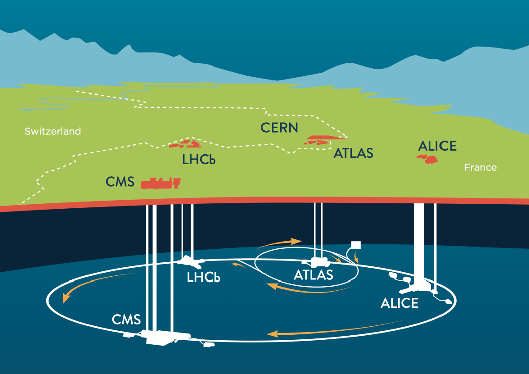
As part of a planned upgrade for the Large Hadron Collider (LHC), a new subdetector named TORCH (Time Of internally Reflected Cherenkov light) is to be added, combining timing information with DIRC-style reconstruction, aiming for a ToF resolution of 10–15 ps (per track).
The DEEPLCEAN3D (DC3D) project focuses on the processing of data once digitised by the TORCH detectors electronics. To retain readability of this document, the specifics of the detector itself and the origin of the data is not discussed in detail, other than a brief overview. As part of this project a full physical simulation of a single TORCH module in operation was created to generate realistic training data. The simulation is hosted as a standalone repository, TORCHSIM on GitHub, which focuses specifically on the detector and the mechanism that produces the data. Check it out for a complete breakdown of the TORCH detector and its operation in the context of the LHCb experiment, if you are unfamiliar with TORCH then this is recommended to fully understand the rest of this document.
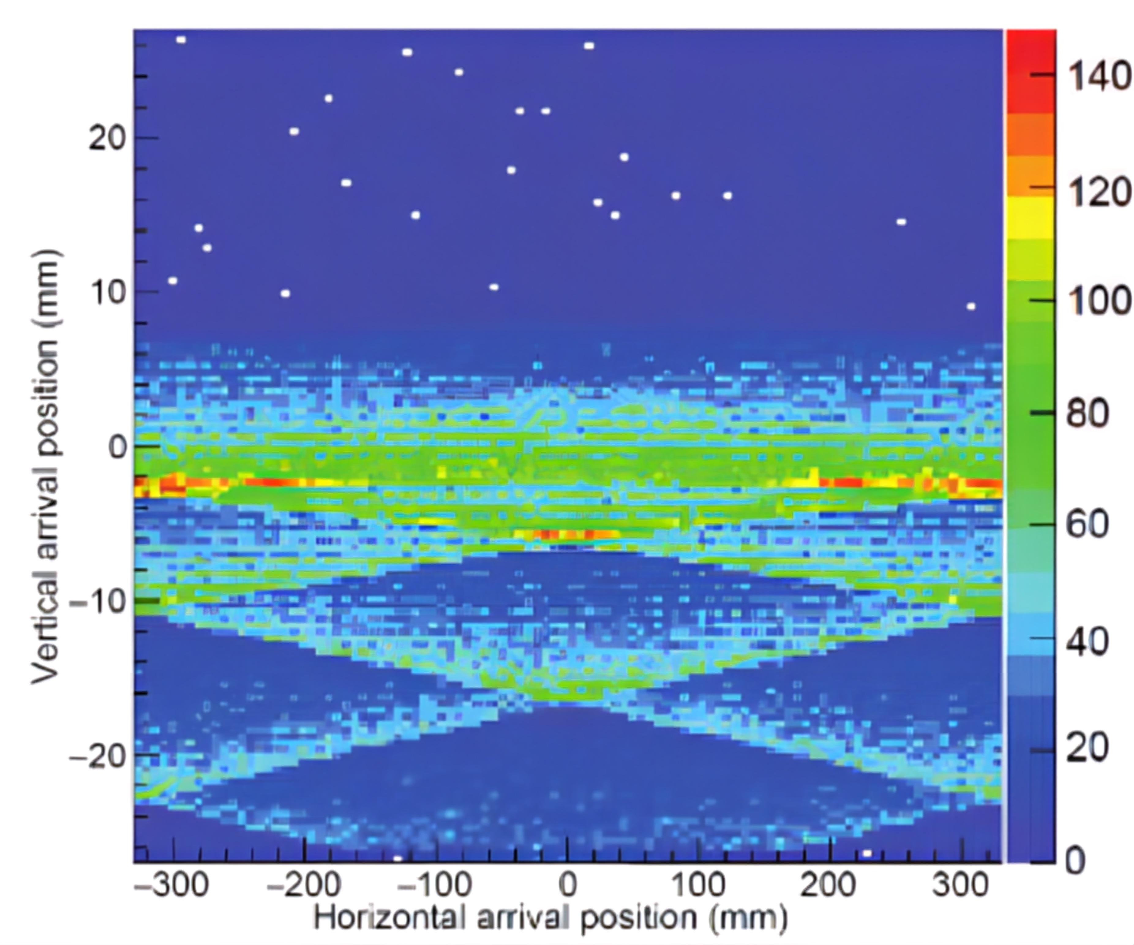
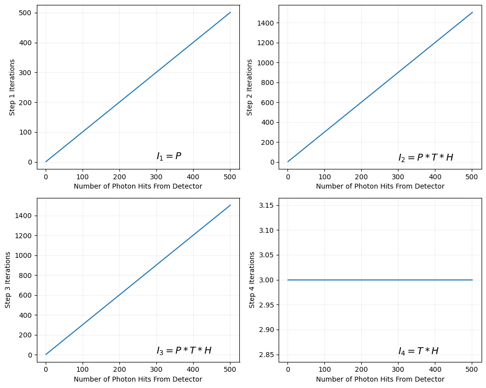
The TORCH subdetector is made up of a bank of photon-multiplier tubes (PMTs), which are sensitive to incoming photons, arranged in a grid/array format. These operate similarly to pixels of a cameras CCD only much faster, with time resolution of approximately 50ps, which in camera talk translates to a 'frame rate' of twenty billion frames per second. The PMTs record the pixel position and the Time-of-Arrival (ToA) of the photons that hit. The purpose of TORCH is to measure the velocity of particles produced in the LHCb experiment, from which particle identity can be inferred. To do this, the path that each photon took through the detector must be reconstructed from the data recorded, a computationally costly process that scales linearly with the number of photons detected. Once all photon paths are reconstructed, only those that are correlated to a particular event are used, the rest are discarded. The discarded photons are typically overlapping tracks or detector noise and constitute around 80% of the total number of photons. After the planned upgrades the LHCb detector is expected to produce up to 500 Tb of data per second, which will be processed in real time, so streamlining the reconstruction process is of maximum importance.
DC3D aims to remove uncorrelated photons from the PMT array data pre-reconstruction, without the benefit of photons path and origin having been calculated. A neural network was developed in PyTorch to achieve this goal The main novel elements presented are in how the data is pre/post-processed, key features and methods employed are outlined in this document. The three main criteria we set out are; decreasing the uncorrelated photons in the data, to not discard or degrade the true correlated photons x, y or ToF values and finally minimal introduction of false positives via processing artefacts that counteract the reduction in noise and could confuse the reconstruction algorithm. Results so far have demonstrated ~91% noise removal whilst retaining ~97% percent of signal photons, the work is still in progress and so check back for updates in the near future.
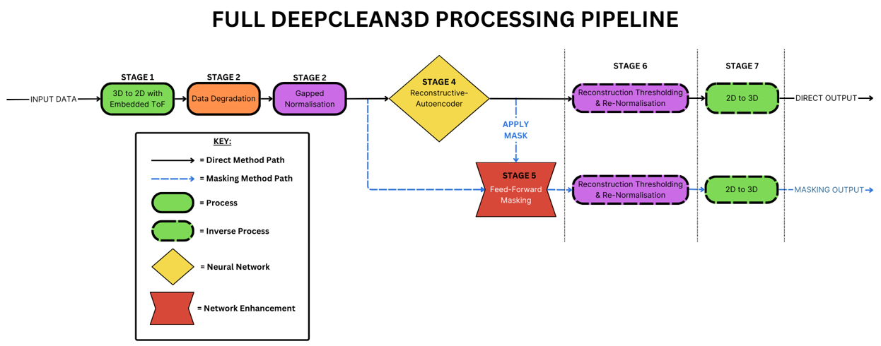
The full DC3D input/output processing pipeline around the central Autoencoder (AE). Data flows from left to right and can take two paths, 'Direct Output' and 'Masking Output'. Each stage is numbered and explained below
To simulates live readout from the detector, the input data is dataset full of 3D arrays of size 128 x 88 x time_step, where time_step is currently 1000.
Very detailed physical simulations of TORCH have been conducted during its development cycle by the LHCb collaboration. From these simulation we can see the expected data has the form:
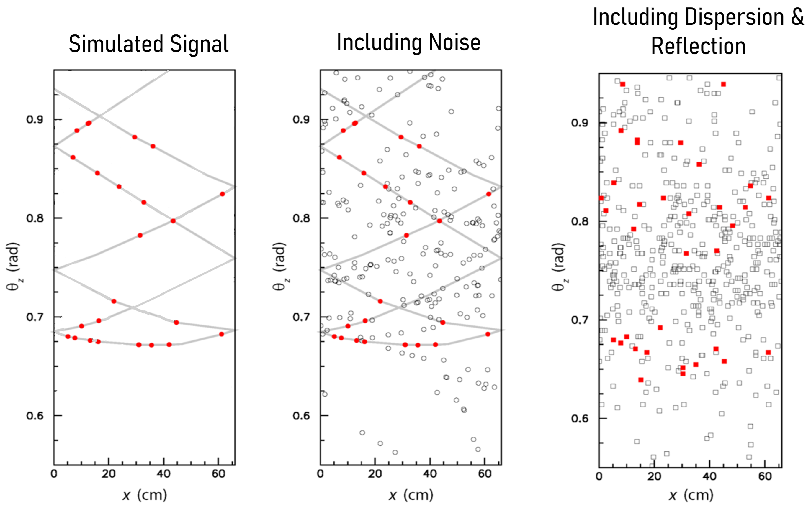
Simulated TORCH data. Background noise points are marked in white, signal points are marked in red and lines joining them up demonstrate the characteristic signal pattern. The left-hand pane shows the simulation without the effects of chromatic dispersion or reflection from the lower edge where the characteristic pattern becomes visible. The right-hand pane shows detector data that includes these effects, the pattern is much harder to make out. TORCH has costly algorithms for correcting for the dispersion and reflection effects, but we hope to automatically correct for them in DC3D
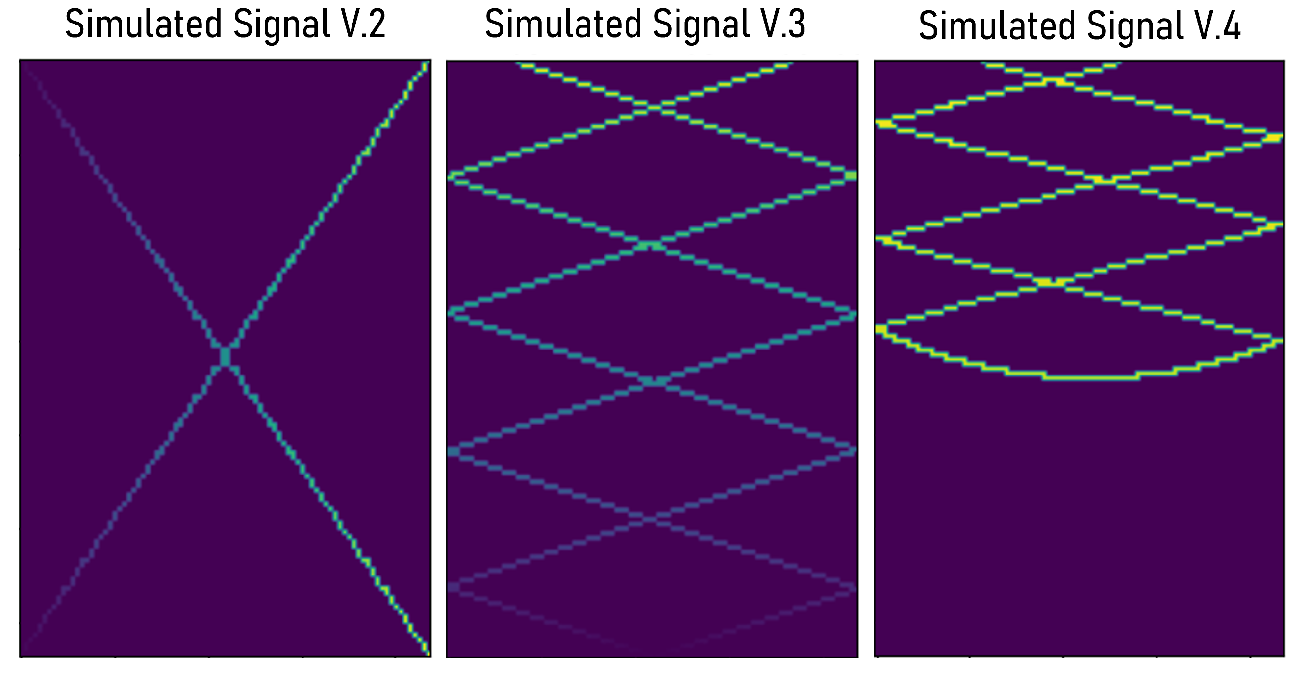
During development of DC3D training data was created with signals patterns of varying degrees of simplification. The stages of signal used in the training data are shown below:
More recently having achieved a good level of performance on the simplified data I have created a physical simulation of a TORCH module in the LHCb detector available via TORCHSIM on GitHub, based on the physical specification set out in the current published literature. The simulation includes the effects of chromatic dispersion and reflection from the lower edge, so we no longer need to simulate these with the degradation functions.
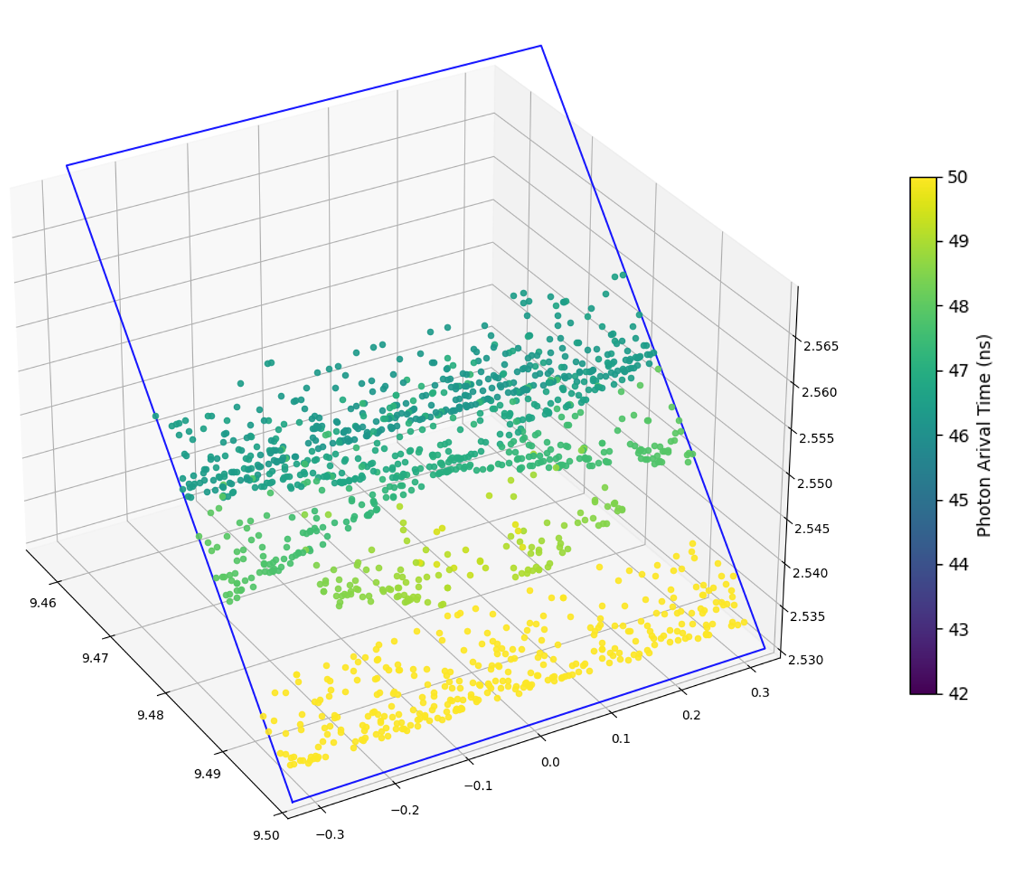
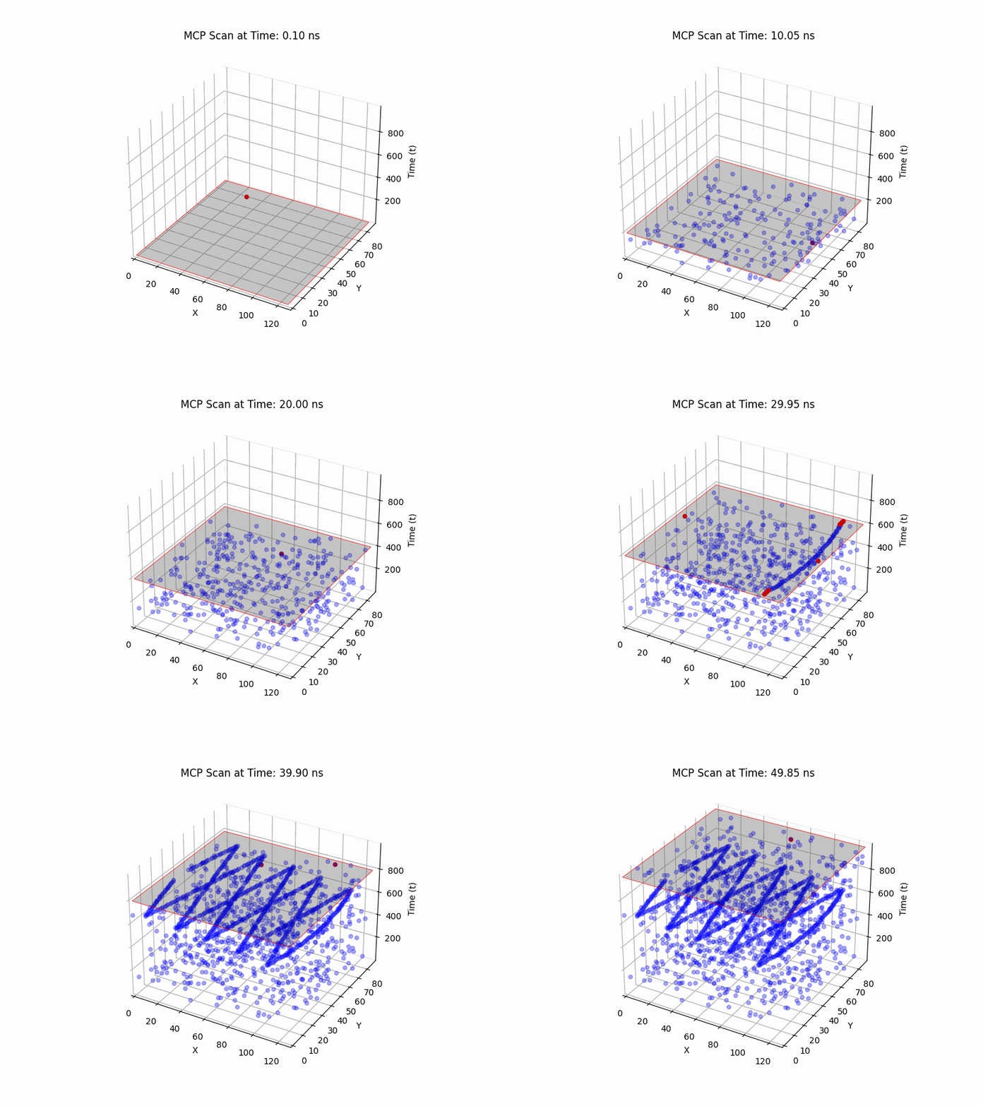
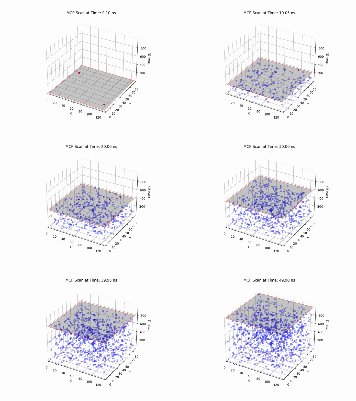
Simplified TORCH data derived from our physically modelled simulation. Simulation available at TORCHSIM on GitHub. Two views of the simulated photon hits on the PMT array, photon number artificially increased to show pattern clearly. The colour of each point shows the time of arrival. The yellow grouping at the bottom of the PMT is the reflection from the bottom edge, the width of the pattern is because of chromatic dispersion. No added background noise is shown.
The initial intention was to make use of 3D convolutions to process the data as a three-dimensional object with x, y and time dimensions. However, it was found to be to computationally intensive. Using the true x, y dimensions of the detector array, 88 x 128 pixels, and a simplified number of time steps 1000 gives 11,264,000 total pixels per 3D image, which results in our autoencoder having 93,411,790 trainable parameters. This is a very large number of parameters, and the training time was found to be prohibitively long. The network was also found to be very sensitive to the number of time steps used, with the number of trainable parameters scaling linearly with the number of time steps. This is a problem as the number of time steps is a key parameter in the TORCH detector design and is not easily changed. The number of time steps is determined by the time resolution of the PMTs and the desired ToF resolution. The number of time steps is currently set to 1000, which is the minimum number of time steps that can be used to achieve the desired ToF resolution of 10-15 ps. The number of time steps is therefore fixed and cannot be optimised.
The solution that was found was to reduce the dimensionality of the input data by squashing the time dimension, leaving a 2D image in X, Y. To retain the time information, we turn the time dimension index of any hit into the value that goes into that x, y position in the 2D array. So instead of a 3D array that has zero values for in place of non-hits and 1's for hits we now have a 2D array with 0's still encoding non hits and now values between 1 and 1000 indicating a hit and the corresponding ToF. This has the effect of reducing the 11m+ total pixels to a more manageable 11,264 and the trainable parameters in the autoencoder to 1,248,251 (an 86.6% decrease over true 3D) which dramatically sped up the processing and training time of the network.
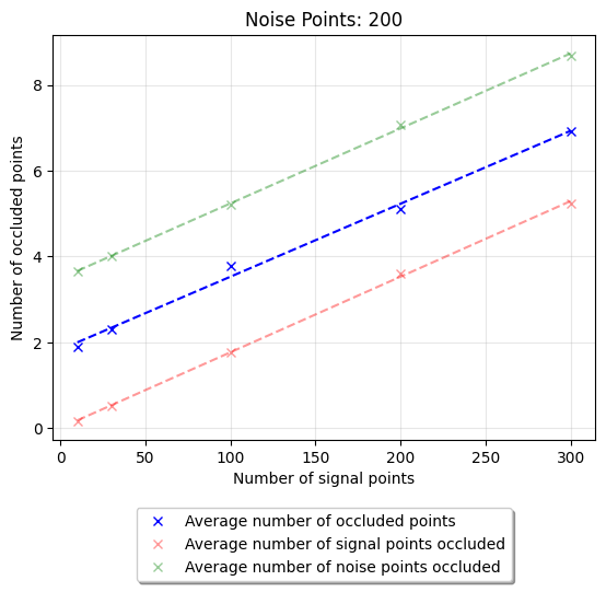
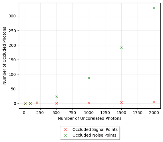
This 2D with embedded ToF approach does introduce two major downsides. Due to the nature of the flattening process it is susceptible to occlusion of pixels, i.e. if there is a noise point with the same x and y position as a signal point but a greater ToF value then it will be the value used in the embedded ToF rather than the signal value behind it. This is not a problem if the amount of noise is not too high. We expect around 30 signal points and 200 noise points distributed over the 11,264 pixels in the squashed 2D image. The probability of a significant portion of the signal being covered up is low, however future improvement and a solution to this occlusion is proposed in section \ref{doublemaskmethod}. Additionally, occlusion effects only the ToF recovery of the signal and not the positional recovery, if a noise point occludes a signal point, then the pattern retains the exact same x, y pixel configuration now with an erroneous ToF value in a pixel. If the signal occludes a noise point it effectively denoises those points. Similarly, if a noise point occludes another noise point this denoises a point. So, the introduced occlusion effect has some possible denoising benefits although they remain unquantified at this time.
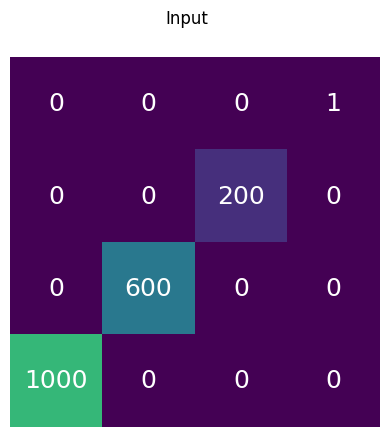
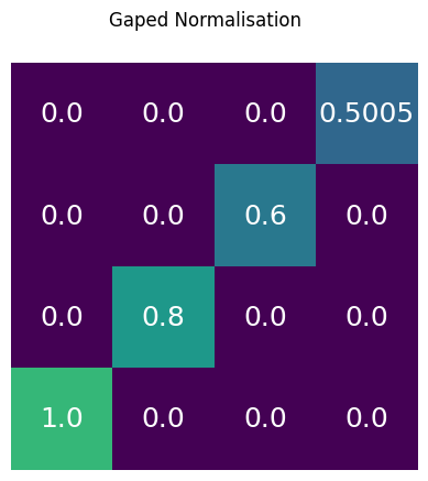
The second issue arising from the 2D with embedded ToF is due to the way the hits are now encoded. The input to the neural network must be normalised to between 0 and 1. In the true 3D network where encoding hits as 0's or 1's there is a clear delineation to the loss function between the two cases. In the 2D embedded method the embedded hits values range from 0 to 1000 and after normalisation the ToF values end up ranging from

Left hand image shows one of the simulated crosses in the full three dimensions of x, y and time. The right-hand side shows the same cross image but using our 2D with embedded ToF method, which compresses the three-dimensional data to two dimensions to speed up the processing.
Stage two of the pipeline is the signal degradation. This is the only stage of the pipeline that is used during training but not during inference. As mentioned in the input data section, each traiing image is a composite of thousands of individual events which fully fills the pattern. From this pure label data we create the 'simulated' degraded input data that will be received by the network in deployment. This includes three steps:
-
Signal removal - The true signal contains many thousands of photons that fill the pattern completely. The network will only receive ~ 30 photons per pattern, so the true signal is thinned out to random values selected from a user input range.
-
Resolution limiting - Next the data is passed through a function that adds a random x and y shift to each photon in the input signal modelled by a Gaussian distribution. This is to simulate the resolution limitations of a detector. We have demonstrated the networks ability to recover the true signal from this degraded input, this has possible application to all detectors and could be used to enhance the physical resolution of a detector through software, an application that we are investigating further in a separate project PLANEBOOST on GitHub.
-
Noise addition - Finally the noise is added to the degraded signal. In more general denoising scenarios the level of noise is sufficiently high that the distribution tends towards a gaussian as described by the central limit theorem. In the case of TORCH, the level of noise is much lower, and the sources are very tightly controlled. For prudence’s sake, the training and inference software includes a variety of noise profiles that can be mixed to create realistic scenarios, which also improves the network generalisation ability. The number of noise pixels added is determined by a user input range. The noise is added to the degraded signal to create the final input image that is passed to the network for denoising.
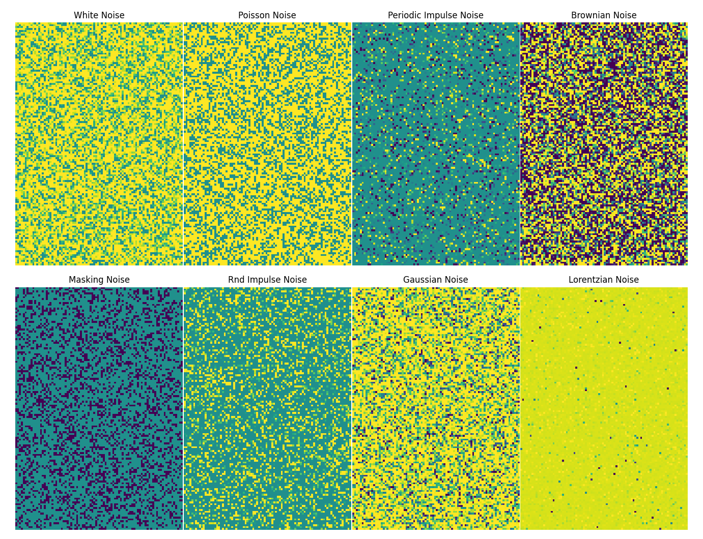
Example of user selectable noise profiles. Amount is exaggerated for clearer representation of subtle differences. Further description is available in the Noise_Generators.py file in the repository.
The way the degradation steps are applied during training is within the main training loop. Therefore, randomised values i.e., number of signal and noise points and the choice of photons selected from the filled label are changed each batch, effectively giving us a near infinite 'virtual dataset' from a small dataset on disk, helping to reduce storage requirements, streamline loading data from disk to memory during training and simplify sending and receiving the datasets during development. This process can also be made fully deterministic is user opts to set a manual seed value in the user settings, and if they have not the random seed values are stored alongside the output so a given virtual dataset can be recalled exactly. This method is possible because each label data file is a composite of many thousands of individual results. Just in the signal points variation alone. The number of possible combinations of 30 signal points from a 2000 point pattern is

Example degradation. Exaggerated number of photons (~300) retained so that the resolution limiting is easily visible. Real data has ~ 30 photons, so much sparser than shown.
A gaped normalisation scheme, eq. \ref{norm eq}, was implemented that aims to create additional separation between non hits and hits, which is especially relevant in the context of our 2D embedded method \ref{2DwToF}. Rather than the standard normalisation that scales an input range from
The reconstruction threshold also allows the data to be reconstructed to 3D without a floor of filed pixels. As we are currently using the output values as a mixture between probabilities and ToF values. something that needs to be addressed!!!!!!!!!!!!!!!!!!!!
The Autoencoder network at the heart of DEEPCLEAN3D is a 9 Layer PyTorch autoencoder with a mixed layer architecture combining the speed and efficiency of convolutional layers with the power of fully connected layers around the latent space. The autoencoder makes use of ReLu activations to protect from exploding/vanishing gradients and employs dropout layers to encourage generalisation and stave off overfitting. The network training environment is developed in Python and allows for automatic hyperparameter optimisation whilst also collecting full detailed telemetry and comparative results for further analysis. The network utilised the powerful ADAM optimiser which uses a momentum term to smooth out the optimization process and adapts the learning rate for each trainable parameter based on its historical gradient. The network is extreamlly computationally lightweight, all included results have been taken while conducting training and inference on an outdated consumer Intel-i7 8700K CPU, with no GPU/Tensor acceleration. The network is designed to be easily scalable to larger and more complex infrastructure and is fully CUDA ready for systems with GPU acceleration available, or deployment in a distributed environment. A particular challenge found in early testing was a lot of false positive hits along the right and bottom edges of the output images, this was found to be caused by a combination of our input shape and the convoloution kernal stride, the network incorperates a special four pixel padding that is added round the entire input and then removed before the final output which fixed the edge distortions. The exact network structure has changed over developent and remains in flux, a full breakdown of the current network structure is available in the XXXXXXXXXXXXXXXXXXXXXXXXXXXXXXXX
During development the network often only returned blank images. After some research and investigation, the problem was found to be an effect known as class imbalance which is an issue that can arise where the interesting features are contained in the minority class \cite{chawla2002smote}. The input image contains 11,264 total pixels and around 230 of them are hits (signal and noise) leaving 98.2% of pixels as non-hits. For the network, just guessing that all the pixels are non-hits yields a 98.2% reconstruction loss and it can easily get stuck in this local minimum.
Class imbalance most commonly appears in classification tasks such as recognising that an image is of a certain class, i.e., ‘cat’, ‘dog', etc. Classification networks often use cross entropy loss and there are specific modifications of it developed to combat class imbalance, such as focal loss \cite{lin2017focal}, Lovász-Softmax\cite{berman2018lovasz} and class-balanced loss \cite{cui2019class}. We present a new similar method called 'Automatic Class Balanced MSE' (ACB-MSE) which instead, through simple modification of the MSE loss function, provides automatic class balancing for MSE loss with additional user adjustable weighting to further tune the networks response. The function relies on the knowledge of the indices for all hits and non-hits in the true label image, which are then compared to the values in the corresponding indices in the recovered image. The loss function is given by:
where
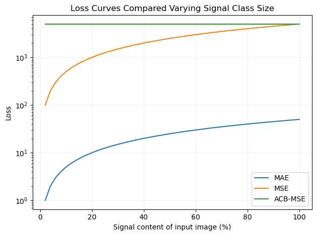
Figure that demonstrates how each of the loss functions (ACB-MSE, MSE and MAE) behave based on the number of hits in the true signal. Two dummy images were created, the first image contains some ToF values of 100 the second image is a replica of the first but only containing the Tof values in half of the number of pixels of the first image, this simulates a 50% signal recovery. to generate the plot the first image was filled in two pixel increments with the second image following at a constant 50% recovery, and at each iteration the loss functions are calculated for the pair of images. We can see how the MSE and MAE functions loss varies as the size of the signal is increased. Whereas the ACB-MSE loss stays constant regardless of the frequency of the signal class.
The loss functions response curve is demonstrated in fig \ref{fig:losscurves}. This shows how the ACB-MSE compares to vanilla MSE and MAE. The addition of ACB balancing means that the separate classes (non-hits and hits) are exactly balanced regardless of how large a proportion of the population they are. this means that by guessing all the pixels are non-hits results in a loss of 50% rather than 98.2%, and to improve on this the network must begin to fill in signal pixels. This frees the network from the local minima of returning blank images and incentives it to put forward its best signal prediction. The addition of the ACB-MSE Loss finally resulted in networks that were able to recover and effectively denoise the input data. The resulting x, y position of the output pixels was measured to be very good and visually the networks were doing a good job of getting close to the right ToF, however, qualitative analysis revealed that the number of pixels with a true ToF value correctly returned was close to zero. To remedy this a novel technique was developed, referred to as 'masking'.
Development was focused on the fully filled out cross patterns with around 200 signal points in this early stage to create a strong proof of concept for the general approach. Feeling like this goal had been achieved the data generator was changed to resemble a more realistic scenario displaying only 30 signal points of the 200 along the cross. The AE developed to this point was not able to learn the sparse patterns.
Taking inspiration from the ideas behind the DAE and how the network is fed idealised data as a label whist it has noised data presented to it, a new methodology was trialled. The input data was reverted to the fully filled 200 photon cross paths, and additional signal degradation methods were incorporated into the noising phase. The initial trial added a function to dropout lit pixels from the input at random till 30 remain, the network is therefore presented with inputs that contain 30 hits only but gets the full filled cross as the label to compute loss against. This works spectacularly well with the network able to accurately reconstruct the patterns from only 30 signal points whilst also still performing the denoising role. This method returns the full cross pattern rather than the specific photon hits that were in the spare input, however if the latter is desired, then the masking method applied to this path results in just the spares photons that fall underneath it in the sparse input image.
For a final experiment into the possibilities of this reconstructive methodology another degradation layer was Incorporated that adds a random x and y shift to each photon in the input signal modelled by a Gaussian distribution. This is to simulate the resolution limitations of a detector. The network is passed in as input an image with all the photon hits shifted and has the perfect image as its label data for loss calculation, this again shows to be a highly successful methodology and demonstrated an ability to produce a tighter output cross signal than the smeared input. This has application to all detectors and could be used to enhance the physical resolution of a detector through software.
This takes us beyond the DAE to a new structure that could be thought of as a Reconstructive Autoencoder or RAE. Like a DAE it aims to learn the underlying pattern behind a noised set of data and then attempt to recreate the label target from the noised samples, but in addition to this the RAE can also reconstruct the signal from a degraded set of measurements.

*Demonstrating the culmination of the RAE with masking applied to a realistic proportion of 30 signal points and 200 noise points. When using the reconstructive method, the direct denoiser output returns the full traced pattern paths which may or may not be of more value than the individual photon hit locations. If this is not the case, then the masking method provides a perfect way to recover the exact signal hits only. *
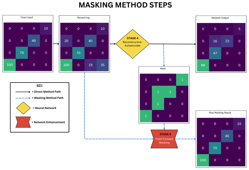
Illustration of the masking technique developed, shown here for a simple 4x4 input image. The numbers in the centre of the squares indicate the pixel values. The colours just help to visualise these values. The blue arrow path is the standard path for the denoising autoencoder, the red path shows the additional masking steps. the green arrow shows where the mask is taken from the standard autoencoders output and cast over the masking paths input.
In the traditional approach and what shall be referred to as the 'direct' method the final denoised output is obtained by taking a clean input image, adding noise to it to simulate the detector noise, then passing the noised image as input to the DC3D denoiser, which removes most of the noise points and produces the finished denoised image. Although the network produces good x, y reconstruction (demonstrated in section \ref{XXXX}RESULTS at 91%), and visually the ToF reconstruction is improving to the point that the signal can be visually discerned when compared to the original as shown in fig \ref{FIGURE OF VUSAL TOF BAD DIRECT}, quantitative analysis reveals that the direct output of the network achieves on average 0% accuracy at finding exact ToF values. To address this problem, we introduce a new technique called ‘masking’.
The 'masking' method introduces an additional step to the process. Instead of taking the output of the denoiser as the final image, this becomes the 'mask'. The mask is then used on the original noised input image using a process described by equation \ref{masking eq}.
where
If the mask has a zero value in an index position, then the noised input is set to zero in that same index which has the effect of removing the noise. If the mask has a non-zero value in it then the value from the corresponding index from the noised input stays as it is, so hits return to having their correct ToF, uncorrupted by the network. An additional benefit of this method is that any additional false positive lit pixels caused by the denoising process will be in the mask and so allow the original value to pass untouched, but the original value in the noised array will be 0 as these points were created by the denoising and so the final output is also automatically cleaned of the majority of denoising artefacts. The two methods are illustrated in fig. \ref{fig:maskingmethod} which shows the direct path in blue arrows and the masking method steps in red.
The masking technique yields perfect ToF recovery for all true signal pixel found, raising ToF recovery from zero to matching the true pixel recovery rate. Computationally, the additional step of casting the mask on the input image to create the masked output is very small compared to the denoising step. To demonstrate this, we timed the two methods (direct denoising vs. denoising + masking) on 1000 test images. The lowest measured run-time for direct denoising was 108.94 ms, and for denoising + masking was 110.29 ms, a 1.24% increase.

Shows the 3D reconstruction for the DAE results with masking. The 3D allows the ToF benefits of the masking to be seen properly. This test featured 200 signal points, and a high amount of noise, 1000 points.
A corresponding re-normalisation function, eq.\ref{renorm eq}, was created that carries out the inverse of the gaped normalisation and is used to transform the networks ToF output back to the original range pre-normalisation. Data values below the reconstruction threshold
In equations \ref{norm eq} and \ref{renorm eq},
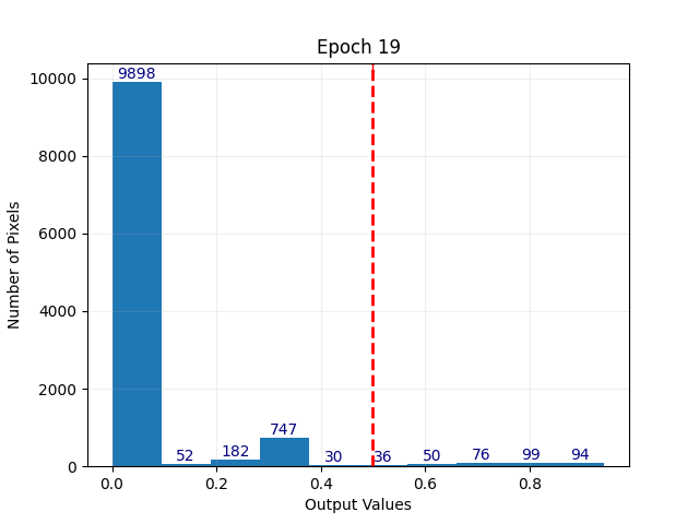
The histogram shows the ToF values for all the pixels in the networks raw output before re-normalisation. Values are between 0 and 1 which is shown on the x axis, the number of pixels in each bin are label on the top of each histogram bin. The red line indicates the reconstruction cutoff value, $r$, All points below this cutoff will be set to 0's in the re-normalisation and all points above it will be spread out into the range 1-100 to return the real ToF value.
Sample overview of results up to this point.
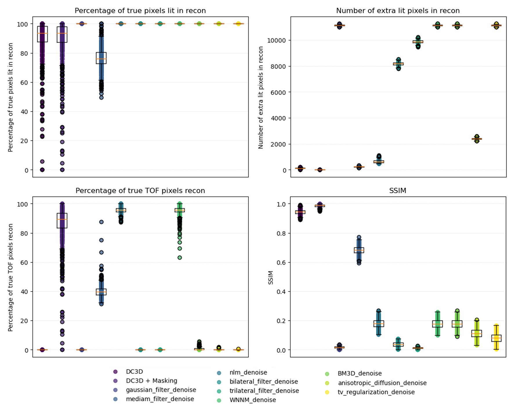
Comparison between DC3D in both normal and masking mode against a range of other popular denoising algorythms both classicalk and neural models i.e the popular BM3D.
Talk performance results
Talk performance results
Talk performance results
Overall including the 2D with embedded ToF technique and the encoder stage the input data has been compressed from 1,126,400 values (an 8MB file when saved to disk in a .npy container) to just 10 numbers (0.000208Mb as a .npy) which itself could have interesting applications. This encoded data would allow for much faster transfer of data allowing processing to be moved further from the detector, or much reduced data storage requirements. The encoded data could be stored so that individual results can be recalled in full using the decoder if they turn out to be of interest later. There is also the exciting possibility of being able to conduct some processing on the data in its encoded form which is another area we are currently investigating with preliminary results to be released in early 2024.
The training speed can be greatly sped up through a variety of low hanging fruit. PyTorch supports CUDA acceleration via GPU’s which is already coded into DC3D as an option, but was not used as the hardware was unavailable. The trainer is also currently optimised for data and telemetry collection rather than efficiency and performance, there remains a large amount of performance to be unlocked by removing the telemetry post development. The PyTorch library back-end is implemented in C++ for speed, but the DC3D front end which handles the data importing and pre and post processing is built in Python for ease of design. The back end makes uses of as much torch and numpy processing as possible but there should be performance gains found from moving to a fully C++ font end, that would allow more control over the underlying hardware.
Currently the autoencoder is optimised to create the best reconstruction it can in all three dimensions. This is then operated on by the masking process as to demonstrate its ability to improve the raw network output. However, if the autoencoder itself was optimised for the masking method rather than its own output there will be a great accuracy improvement as the network will now only have to deal with classifying pixels as on or off, which removes the added complexity of the gaped normalisation and re-normalisation routines as well creating the greatest distance between signal and non-signal points aiding the network in its reconstruction.
Another possibility to improve the networks recovery performance would be to implement double masking, where one mask is created by the autoencoder working on the data flattened to the x,y plane and another is calculated form the data flattened to the x, time plane, this would give two views into the 3d data which would help to mitigate the occlusion issue caused by the 2D with embedded ToF method whilst also hopefully bringing the networks good x,y location performance to the ToF data. The difficulty and still an open question needing further research is how the two masking views results will be combined/processed to determine the final output.
A flaw in our initial testing methodology comes from the long training time for each model. Therefore, during the initial settings optimisation a happy medium of 15 epochs was settled on for the training time. This could have biased the chosen parameters towards those that enable the neural network to learn a good representation fast but maybe away from those that would enable it to find the best reconstruction possible. This could be remedied through additional compute hardware or deploying the model training on cloud based infrastructure allowing for much longer testing to find the optimum settings for performance rather than training speed. If you are in a position to provide access to CUDA compute for the project to expand this testing please do get in touch!
This project is not currently licensed. The ACB-MSE loss function is licensed under the MIT License and is available at ACB-MSE repository and via PyPi.
Contributions to this codebase are welcome! If you encounter any issues, bugs or have suggestions for improvements please open an issue or a pull request on the GitHub repository.
For any further inquiries or for assistance in deploying DC3D, please feel free to reach out to me at adill@neuralworkx.com.
Special thanks to Professor Jonas Radamaker for his guidance and expertise on LHCb and the TORCH project, Dr Alex Marshall for his support and troubleshooting, and Max Carter for his contributions and signal generator used in early development.
[1] LHCb Collaboration et al. Evidence for cp violation in time-integrated d0→ h- h+ decay rates. Physical Review Letters, 2012, Vol. 108, No. 11, 2012.
[2] Paul Langacker. The standard model and beyond. Taylor & Francis, 2017.
[3] Roel Aaij, B Adeva, M Adinolfi, A Affolder, Z Ajaltouni, S Akar, J Albrecht, F Alessio, M Alexander, S Ali, et al. Evidence for c p violation in b+→ p p¯ k+ decays. Physical review letters, 113(14):141801, 2014.
[4] LHCb Collaboration et al. Measurement of the bs0→ µ+ µ-branching fraction and effective lifetime and search for b0→ µ+ µ-decays. Physical Review Letters, 118(19):191801, 2017.
[5] Bockelman et al. Iris-hep strategic plan for the next phase of software upgrades for hl-lhc physics. Technical report, 2023.
[6] ATLAS collaboration et al. Atlas software and computing hl-lhc roadmap. Technical report, 2022.
[7] LHCb Collaboration, CERN (Meyrin). Framework TDR for the LHCb Upgrade II Opportunities in flavour physics, and beyond, in the HL-LHC era. Technical report, CERN, Geneva, 2021.
[8] Neville Harnew, R Gao, T Hadavizadeh, TH Hancock, JC Smallwood, NH Brook, S Bhasin, D Cussans, J Rademacker, R Forty, et al. The torch time-of-flight detector. Nuclear Instruments and Methods in Physics Research Section A: Accelerators, Spectrometers, Detectors and Associated Equipment, 1048:167991, 2023.
[9] I Bediaga, M Cruz Torres, JM De Miranda, A Gomes, A Massafferri, J Molina Rodriguez, AC dos Reis, R Aoude, S Amato, K Carvalho Akiba, et al. Physics case for an lhcb upgrade ii-opportunities in flavour physics, and beyond, in the hl-lhc era. arXiv preprint arXiv:1808.08865, 2018.
[10] MJ Charles, R Forty, LHCb Collaboration, et al. Torch: Time of flight identification with cherenkov radiation. Nuclear Instruments and Methods in Physics Research Section A: Accelerators, Spectrometers, Detectors and Associated Equipment, 639(1):173–176, 2011.
[11] JC Smallwood, S Bhasin, T Blake, NH Brook, MF Cicala, T Conneely, D Cussans, MWU van Dijk, R Forty, C Frei, et al. Test-beam demonstration of a torch prototype module. In Journal of Physics: Conference Series, volume 2374, page 012004. IOP Publishing, 2022.
[12] Maarten Van Dijk. Design of the TORCH detector: A Cherenkov based Time-of-Flight system for particle identification. PhD thesis, Oxford U., 2016.
[13] Vitalii L Ginzburg. Radiation by uniformly moving sources (vavilov–cherenkov effect, transition radiation, and other phenomena). Physics-Uspekhi, 39(10):973, 1996.
[14] Boris M Bolotovskii. Vavilov–cherenkov radiation: its discovery and application. Physics-Uspekhi, 52(11):1099,
[15] Robert W Boyd and Daniel J Gauthier. Slow and fast light. 2002.
[16] Maria Flavia Cicala, Srishti Bhasin, Thomas Blake, Nick H Brook, Thomas Conneely, David Cussans, Maarten WU van Dijk, Roger Forty, Christoph Frei, Emmy PM Gabriel, et al. Picosecond timing of charged particles using the torch detector. Nuclear Instruments and Methods in Physics Research Section A: Accelerators, Spectrometers, Detectors and Associated Equipment, 1038:166950, 2022.
[17] Jonas Rademacker. Torch reconstruction. Technical report, 2022.
[18] H Merritt. Detectors of internally reflected cherenkov light. 2009.
[19] R Gao, N Brook, L Castillo Garc´ıa, D Cussans, K Fohl, R Forty, C Frei, T Gys, N Harnew, D Piedigrossi, et al. Development of torch readout electronics for customised mcps. Journal of Instrumentation, 11(04):C04012, 2016.
[20] Roger Forty. The torch project. Journal of Instrumentation, 9(04):C04024, 2014.
[21] Neville Harnew. Torch: A large-area detector for precision time-of-flight measurements at lhcb. Physics Procedia, 37:626–633, 2012.
[22] T Jones, S Bhasin, T Blake, NH Brook, MF Cicala, T Conneely, D Cussans, MWU van Dijk, R Forty, C Frei, et al. New developments from the torch r&d project. Nuclear Instruments and Methods in Physics Research Section A: Accelerators, Spectrometers, Detectors and Associated Equipment, 1045:167535, 2023.
[23] Klaus Fohl. TORCH — an Innovative High-Precision Time-of-Flight PID Detector for the LHCb Upgrade. page 7431227, 2015.
[24] NH Brook, L Castillo Garc´ıa, TM Conneely, David Cussans, MWU van Dijk, Klaus F¨ohl, Roger Forty, Christoph Frei, Rui Gao, Thierry Gys, et al. Testbeam studies of a torch prototype detector. Nuclear Instruments and Methods in Physics Research Section A: Accelerators, Spectrometers, Detectors and Associated Equipment, 908:256– 268, 2018.
[25] Srishti Bhasin, Roger Forty, Guy Wilkinson, Thomas Blake, Thierry Gys, Silvia Gambetta, Rui Gao, Emmy Pauline Maria Gabriel, Jonas Rademacker, Franz Muheim, et al. Torch physics performance: improving low momentum pid performance during upgrade ib and beyond. Technical report, 2020.
[26] Chunwei Tian, Lunke Fei, Wenxian Zheng, Yong Xu, Wangmeng Zuo, and Chia-Wen Lin. Deep learning on image denoising: An overview. Neural Networks, 131:251–275, 2020.
[27] Kazufumi Ito and Kaiqi Xiong. Gaussian filters for nonlinear filtering problems. IEEE transactions on automatic control, 45(5):910–927, 2000.
[28] Jacob Benesty, Jingdong Chen, and Yiteng Huang. Study of the widely linear wiener filter for noise reduction. In 2010 IEEE International Conference on Acoustics, Speech and Signal Processing, pages 205–208. IEEE, 2010.
[29] Yong Lee and S Kassam. Generalized median filtering and related nonlinear filtering techniques. IEEE Transactions on Acoustics, Speech, and Signal Processing, 33(3):672–683, 1985.
[30] Carlo Tomasi and Roberto Manduchi. Bilateral filtering for gray and color images. In Sixth international conference on computer vision (IEEE Cat. No. 98CH36271), pages 839–846. IEEE, 1998.
[31] Jun Xu, Lei Zhang, and David Zhang. A trilateral weighted sparse coding scheme for real-world image denoising. In Proceedings of the European conference on computer vision (ECCV), pages 20–36, 2018.
[32] Kostadin Dabov, Alessandro Foi, Vladimir Katkovnik, and Karen Egiazarian. Image denoising by sparse 3-d transform-domain collaborative filtering. IEEE Transactions on image processing, 16(8):2080–2095, 2007.
[33] Leonid I Rudin, Stanley Osher, and Emad Fatemi. Nonlinear total variation based noise removal algorithms. Physica D: nonlinear phenomena, 60(1-4):259–268, 1992.
[34] Camille Sutour, Charles-Alban Deledalle, and Jean-Fran¸cois Aujol. Adaptive regularization of the nl-means: Application to image and video denoising. IEEE Transactions on image processing, 23(8):3506–3521, 2014.
[35] Linwei Fan, Fan Zhang, Hui Fan, and Caiming Zhang. Brief review of image denoising techniques. Visual Computing for Industry, Biomedicine, and Art, 2(1):1–12, 2019.
[36] Leonid I Rudin and Stanley Osher. Total variation based image restoration with free local constraints. In Proceedings of 1st international conference on image processing, volume 1, pages 31–35. IEEE, 1994.
[37] D Maheswari and V Radha. Noise removal in compound image using median filter. International Journal on Computer Science and Engineering, 2(04):1359–1362, 2010.
[38] Arce and McLoughlin. Theoretical analysis of the max/median filter. IEEE transactions on acoustics, speech, and signal processing, 35(1):60–69, 1987.
[39] Peter Ndajah, Hisakazu Kikuchi, Masahiro Yukawa, Hidenori Watanabe, and Shogo Muramatsu. An investigation on the quality of denoised images. International Journal of Circuit, Systems, and Signal Processing, 5(4):423–434,
[40] Anil K Jain. Fundamentals of digital image processing. Prentice-Hall, Inc., 1989.
[41] Ian Goodfellow, Jean Pouget-Abadie, Mehdi Mirza, Bing Xu, David Warde-Farley, Sherjil Ozair, Aaron Courville, and Yoshua Bengio. Generative adversarial nets. In Advances in neural information processing systems, pages 2672–2680, 2014.
[42] Frank Rosenblatt. The perceptron: a probabilistic model for information storage and organization in the brain. Psychological review, 65(6):386, 1958.
[43] Stefan Leijnen and Fjodor van Veen. The neural network zoo. In Proceedings, volume 47, page 9. MDPI, 2020.
[44] Yann LeCun, Yoshua Bengio, and Geoffrey Hinton. Deep learning. nature, 521(7553):436–444, 2015.
[45] Pascal Vincent, Hugo Larochelle, Yoshua Bengio, and Pierre-Antoine Manzagol. Extracting and composing robust features with denoising autoencoders. In Proceedings of the 25th international conference on Machine learning, pages 1096–1103, 2008.
[46] Kyojin Jang, Seokyoung Hong, Minsu Kim, Jonggeol Na, and Il Moon. Adversarial autoencoder based feature learning for fault detection in industrial processes. IEEE Transactions on Industrial Informatics, 18(2):827–834, 2021.
[47] Yiru Zhao, Bing Deng, Chen Shen, Yao Liu, Hongtao Lu, and Xian-Sheng Hua. Spatio-temporal autoencoder for video anomaly detection. In Proceedings of the 25th ACM international conference on Multimedia, pages 1933–1941, 2017.
[48] Yasi Wang, Hongxun Yao, and Sicheng Zhao. Auto-encoder based dimensionality reduction. Neurocomputing, 184:232–242, 2016.
[49] Joana Frontera-Pons, Florent Sureau, Jerome Bobin, and Emeric Le Floc’h. Unsupervised feature-learning for galaxy seds with denoising autoencoders. Astronomy & Astrophysics, 603:A60, 2017.
[50] Jo Schlemper, Jose Caballero, Joseph V Hajnal, Anthony Price, and Daniel Rueckert. A deep cascade of convolutional neural networks for mr image reconstruction. In Information Processing in Medical Imaging: 25th International Conference, IPMI 2017, Boone, NC, USA, June 25-30, 2017, Proceedings 25, pages 647–658. Springer, 2017.
[51] Xiao Xiang Zhu, Devis Tuia, Lichao Mou, Gui-Song Xia, Liangpei Zhang, Feng Xu, and Friedrich Fraundorfer. Deep learning in remote sensing: A comprehensive review and list of resources. IEEE geoscience and remote sensing magazine, 5(4):8–36, 2017.
[52] Eli Stevens, Luca Antiga, and Thomas Viehmann. Deep learning with PyTorch. Manning Publications, 2020.
[53] Matthew D Zeiler and Rob Fergus. Visualizing and understanding convolutional networks. In Computer Vision– ECCV 2014: 13th European Conference, Zurich, Switzerland, September 6-12, 2014, Proceedings, Part I 13, pages 818–833. Springer, 2014.
[54] Geoffrey E. Hinton, Nitish Srivastava, Alex Krizhevsky, Ilya Sutskever, and Ruslan Salakhutdinov. Improving neural networks by preventing co-adaptation of feature detectors. CoRR, abs/1207.0580, 2012.
[55] Jonathan Tompson, Ross Goroshin, Arjun Jain, Yann LeCun, and Christoph Bregler. Efficient object localization using convolutional networks. In Proceedings of the IEEE conference on computer vision and pattern recognition, pages 648–656, 2015.
[56] Sergey Ioffe and Christian Szegedy. Batch normalization: Accelerating deep network training by reducing internal covariate shift. In International conference on machine learning, pages 448–456. pmlr, 2015.
[57] Vinod Nair and Geoffrey E Hinton. Rectified linear units improve restricted boltzmann machines. In Proceedings of the 27th international conference on machine learning (ICML-10), pages 807–814, 2010.
[58] Alex Krizhevsky, Ilya Sutskever, and Geoffrey E Hinton. Imagenet classification with deep convolutional neural networks. Communications of the ACM, 60(6):84–90, 2017.
[59] Diederik P Kingma and Jimmy Ba. Adam: A method for stochastic optimization. arXiv preprint arXiv:1412.6980, 2014.
[60] Sashank J Reddi, Satyen Kale, and Sanjiv Kumar. On the convergence of adam and beyond. arXiv preprint arXiv:1904.09237, 2019.
[61] Ruo-Yu Sun. Optimization for deep learning: An overview. Journal of the Operations Research Society of China, 8(2):249–294, 2020.
[62] Nitesh V Chawla, Kevin W Bowyer, Lawrence O Hall, and W Philip Kegelmeyer. Smote: synthetic minority over-sampling technique. Journal of artificial intelligence research, 16:321–357, 2002.
[63] Tsung-Yi Lin, Priya Goyal, Ross Girshick, Kaiming He, and Piotr Doll´ar. Focal loss for dense object detection. In Proceedings of the IEEE international conference on computer vision, pages 2980–2988, 2017.
[64] Maxim Berman, Amal Rannen Triki, and Matthew B Blaschko. The lov´asz-softmax loss: A tractable surrogate for the optimization of the intersection-over-union measure in neural networks. In Proceedings of the IEEE conference on computer vision and pattern recognition, pages 4413–4421, 2018.
[65] Yin Cui, Menglin Jia, Tsung-Yi Lin, Yang Song, and Serge Belongie. Class-balanced loss based on effective number of samples. In Proceedings of the IEEE/CVF conference on computer vision and pattern recognition, pages 9268–9277, 2019.
[66] Zhou Wang, Alan C Bovik, Hamid R Sheikh, and Eero P Simoncelli. Image quality assessment: from error visibility to structural similarity. IEEE transactions on image processing, 13(4):600–612, 2004.
[67] Zhou Wang, Eero P Simoncelli, and Alan C Bovik. Multiscale structural similarity for image quality assessment. In The Thrity-Seventh Asilomar Conference on Signals, Systems & Computers, 2003, volume 2, pages 1398–1402. Ieee, 2003.
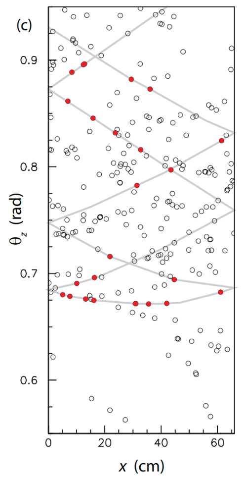
Left-hand image shows the 2d flattened data for many charged hadrons passing the quartz in the centre of the block overlayed. with the colour scale indicating the number of detections per pixel. image source: \cite{brook2018testbeam}. Realistic distribution of photon detections taken for one simulated charged hadron passing through the quartz block. The red pixels indicate the ones that are correlated to the charged hadron. The line joining the red points is an aid for the eye to demonstrate that the signal points fall on the characteristic pattern. Image source: \cite{forty2014torch}.
The number of iterations required for each processing step of the analytical PDF method Vs the number of photons received from the detector. Shown for a single track and with three particle hypothesises, pion/kaon/proton. Each stage's iterations, $I_1$ through to $I_4$ has its function given on the plot in terms of P the number of photons detected, H the number of hypothesis and T the number of tracks.
LHC Ring with the four main experiments shown. Includes the underground detectors and above ground control stations.

The results of the RAE applied to the 30 signal and 200 noise points shown in reconstructed 3D. It is important to note that the masked output does not look like the input image because in the case of the reconstructive method the masking recovers only the true signal points incident on the detector not the full pattern, these points are the input image after it has been thinned out by the sparsity function.
1) 2D with embedded ToF: The detector produces 100, 128 x 88 images these are compressed to a single 128 x 88 image using the 2D with embedded ToF technique.

2) Detector Smearing, Signal Sparsity and Noise are added to the image.

3) Gaped Normalisation: the image is normalised using the gaped normalisation method.

4) RAE: the image is processed by the DC3D Autoencoder network, shown in more detail in section \ref{AEDEEP}.

5) Direct Output: The output of the autoencoder produces the denoised image.

6) if using the direct method this denoised image is the result and is passed to the re-normalisation in step 10.

7) If using the masking method the input to the autoencoder is used as the input for masking.

8) The autoencoders output is used as a mask on the input to recover the correct ToF values.

9) If using the masking method the output of step 8 is the result and is passed to the re-normalisation in step 10.

10) Gaped Re-normalisation: Performs the inverse of the gaped normalisation to recover the ToF values.

11) Inverse 2D with embedded ToF: performs the inverse of the 3D to 2D with embedded ToF to recover the 3D data.


