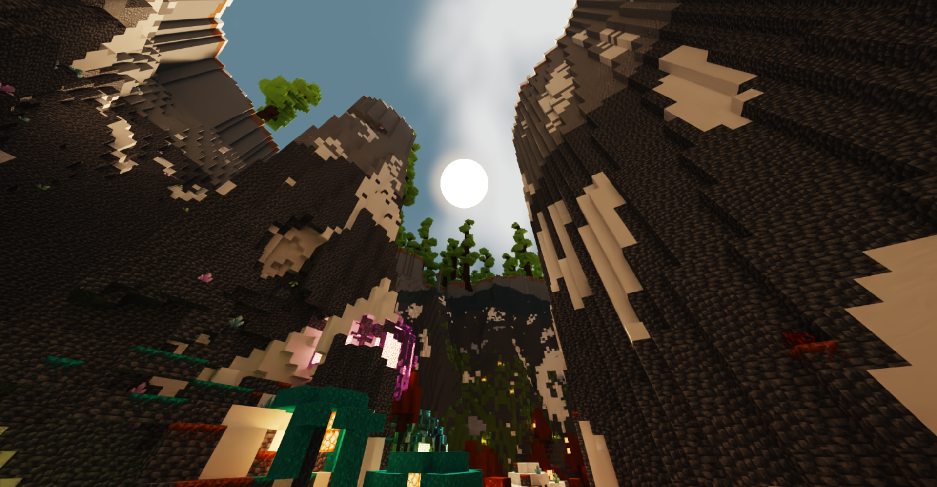
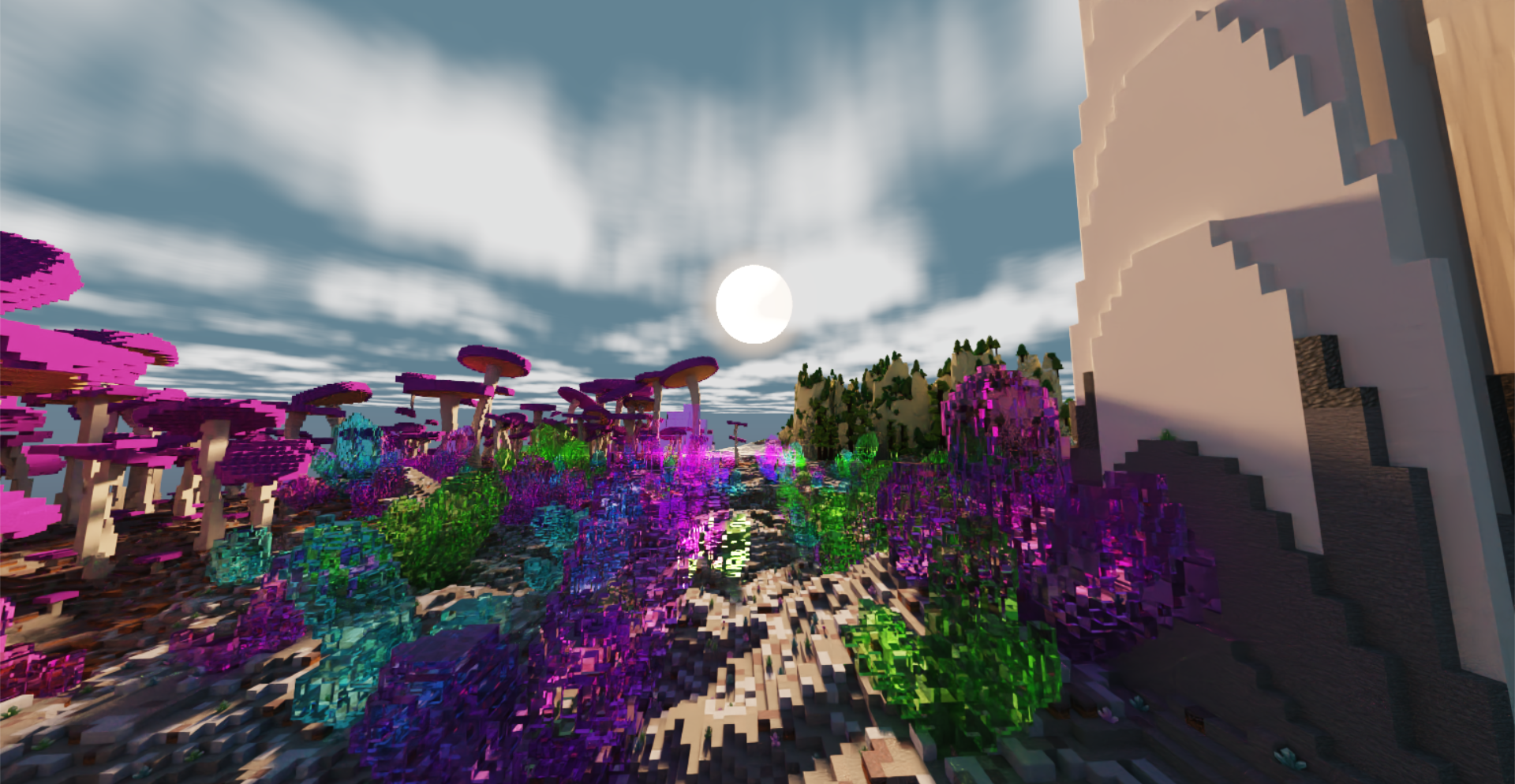
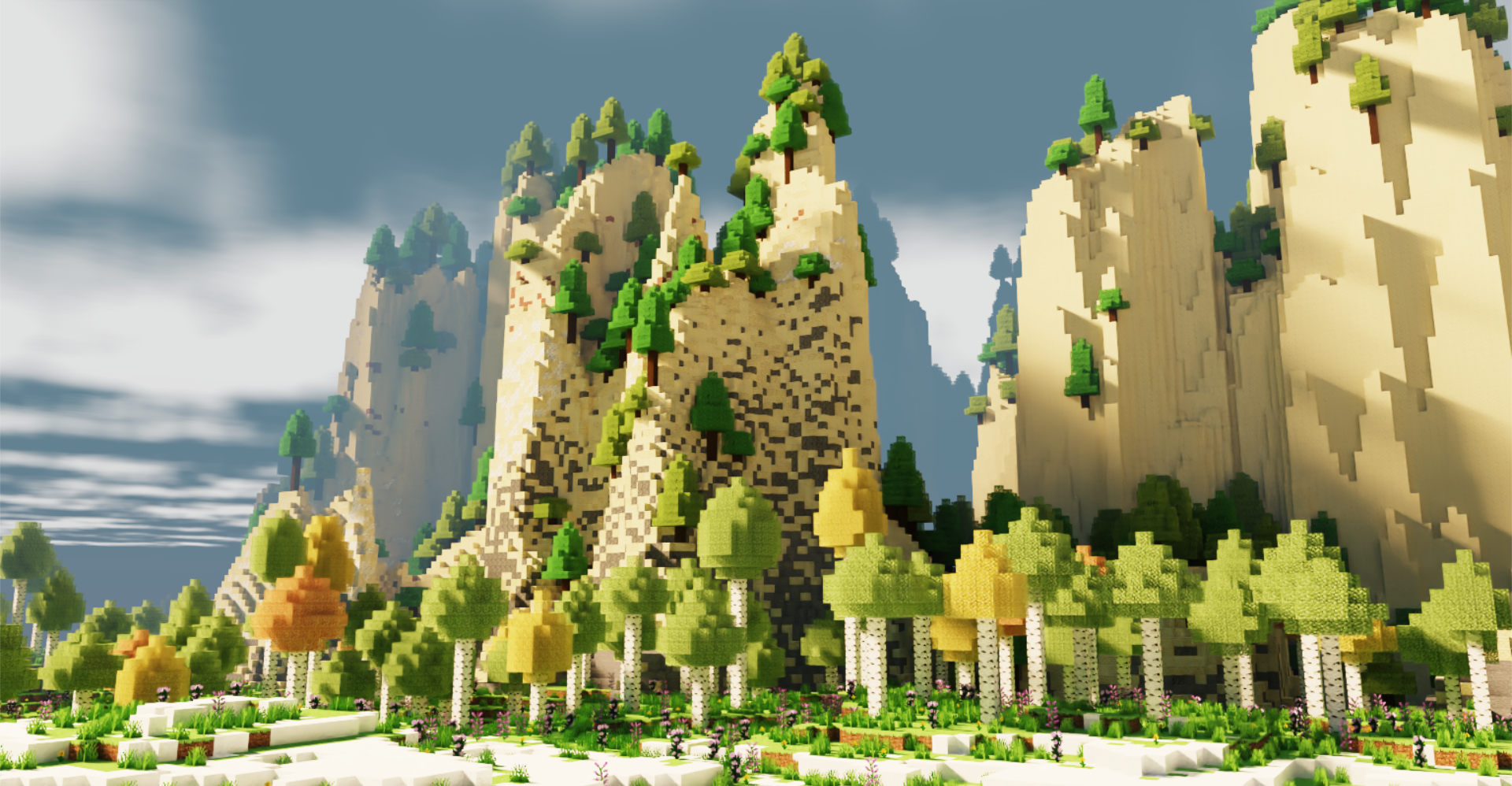
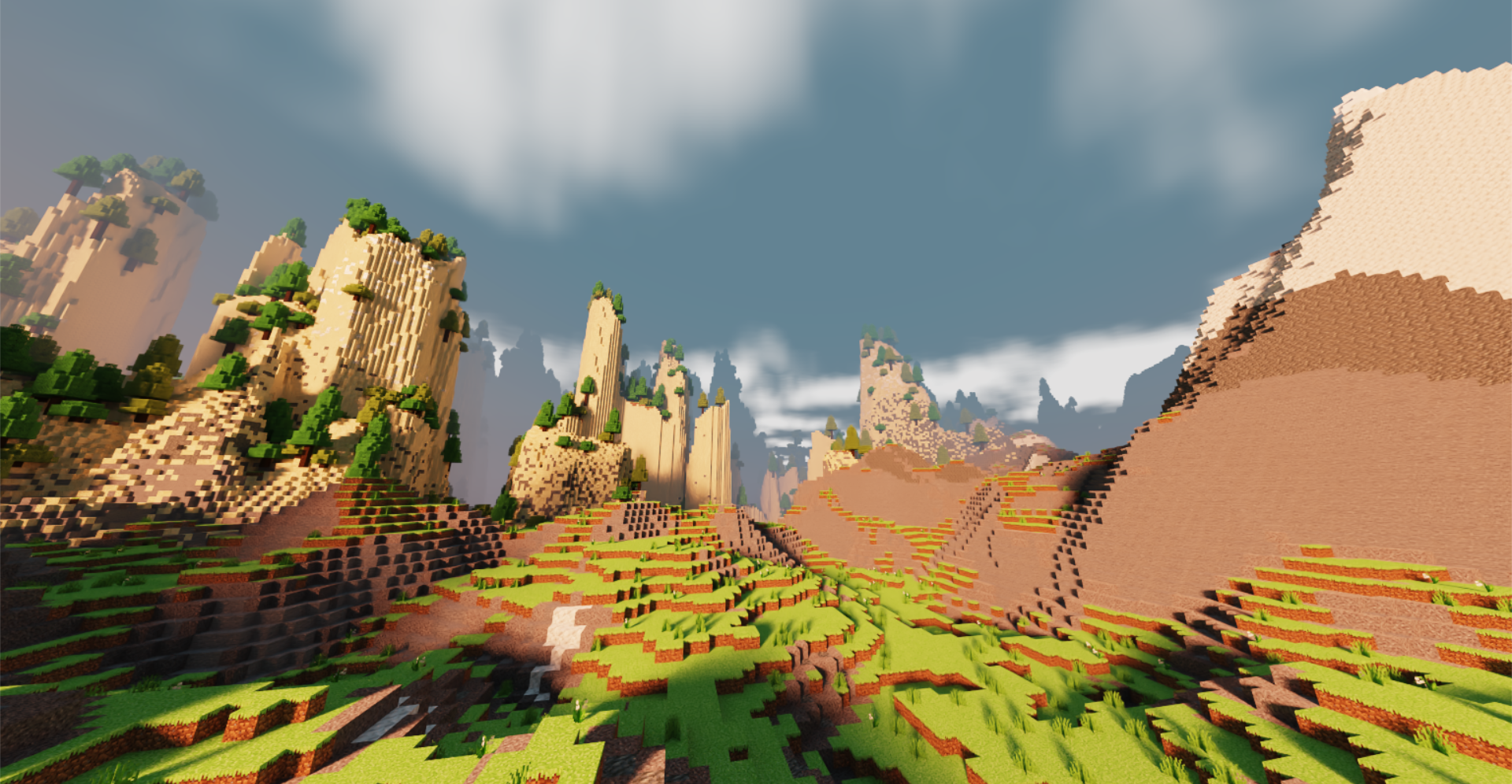
University of Pennsylvania, CIS 565: GPU Programming and Architecture, Final Project
Video demo: https://youtu.be/-jJlK3-Xo-Q
Presentations: pitch, milestone 1, milestone 2, milestone 3, final
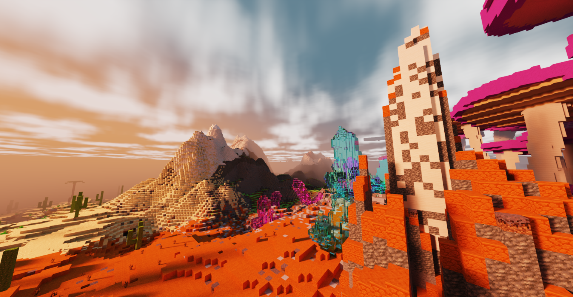
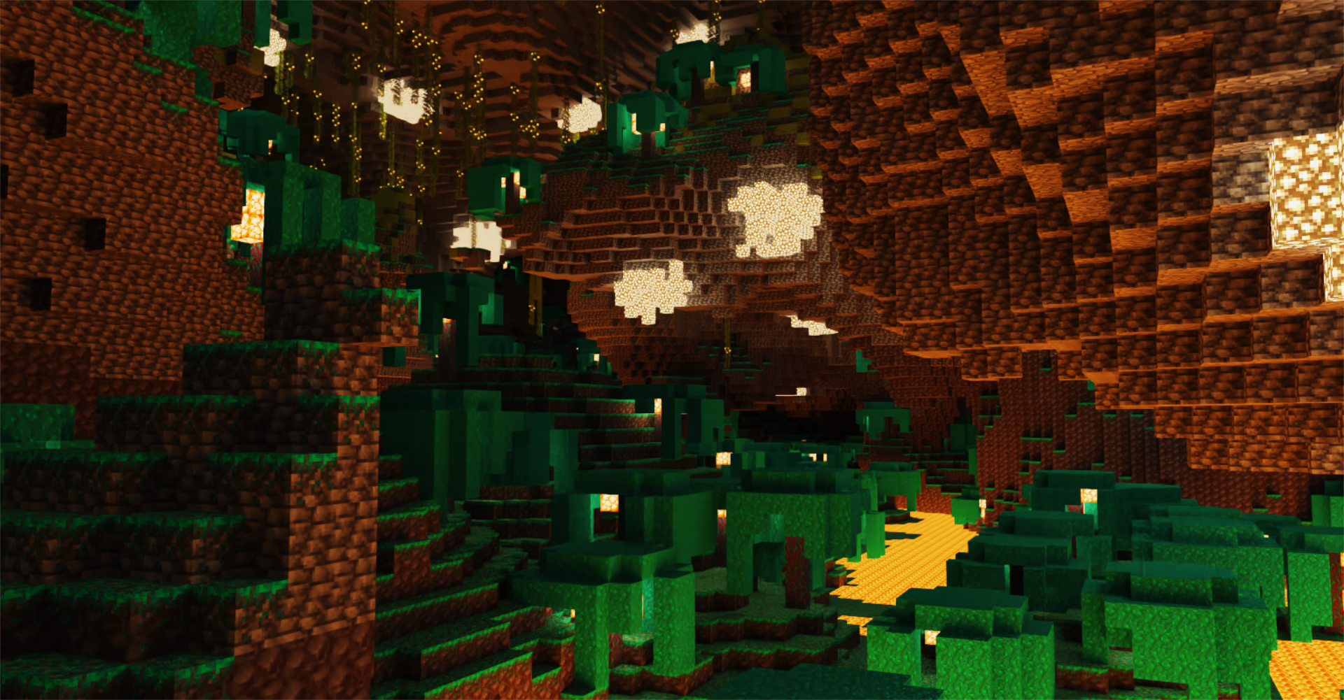
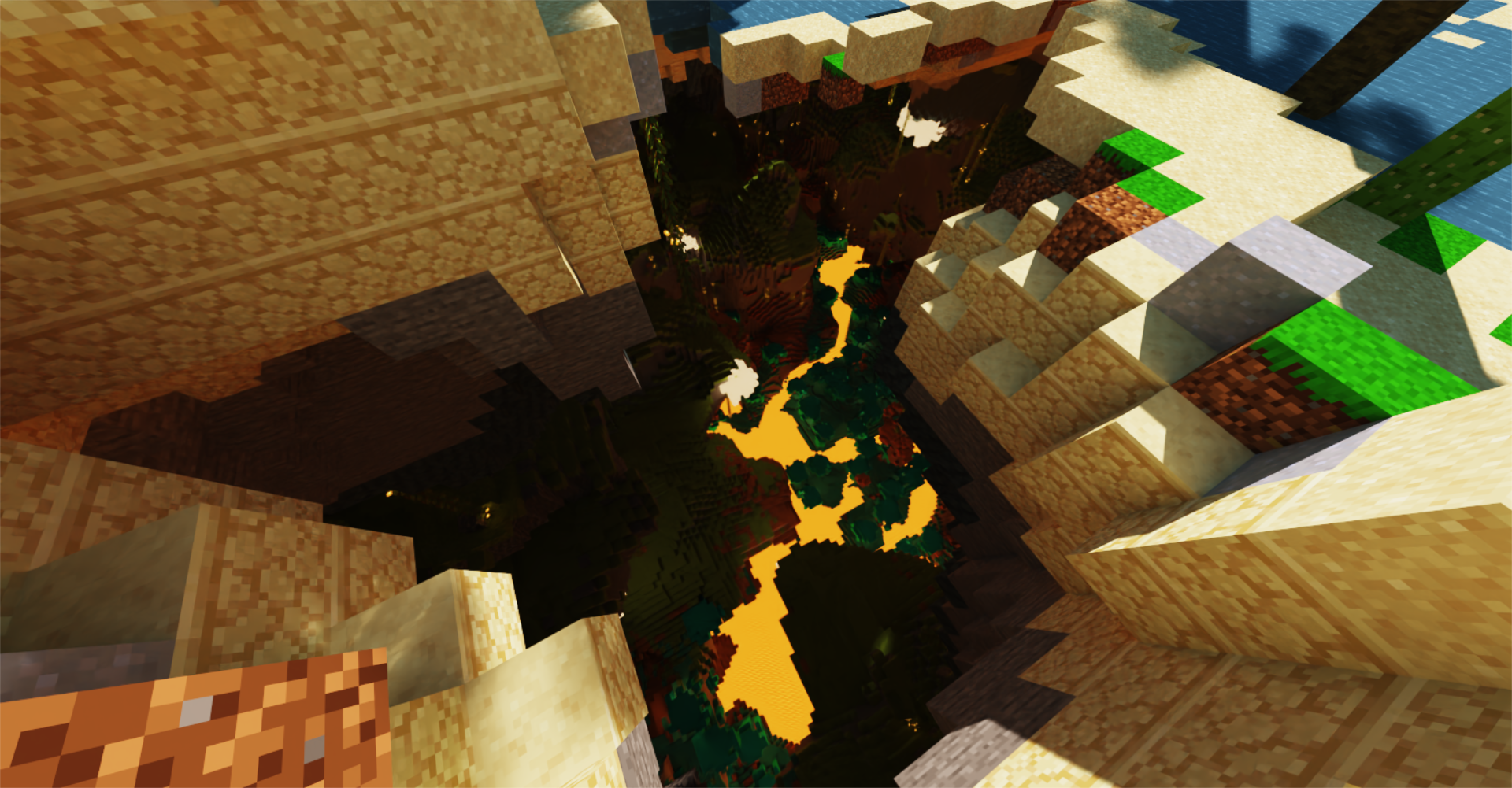
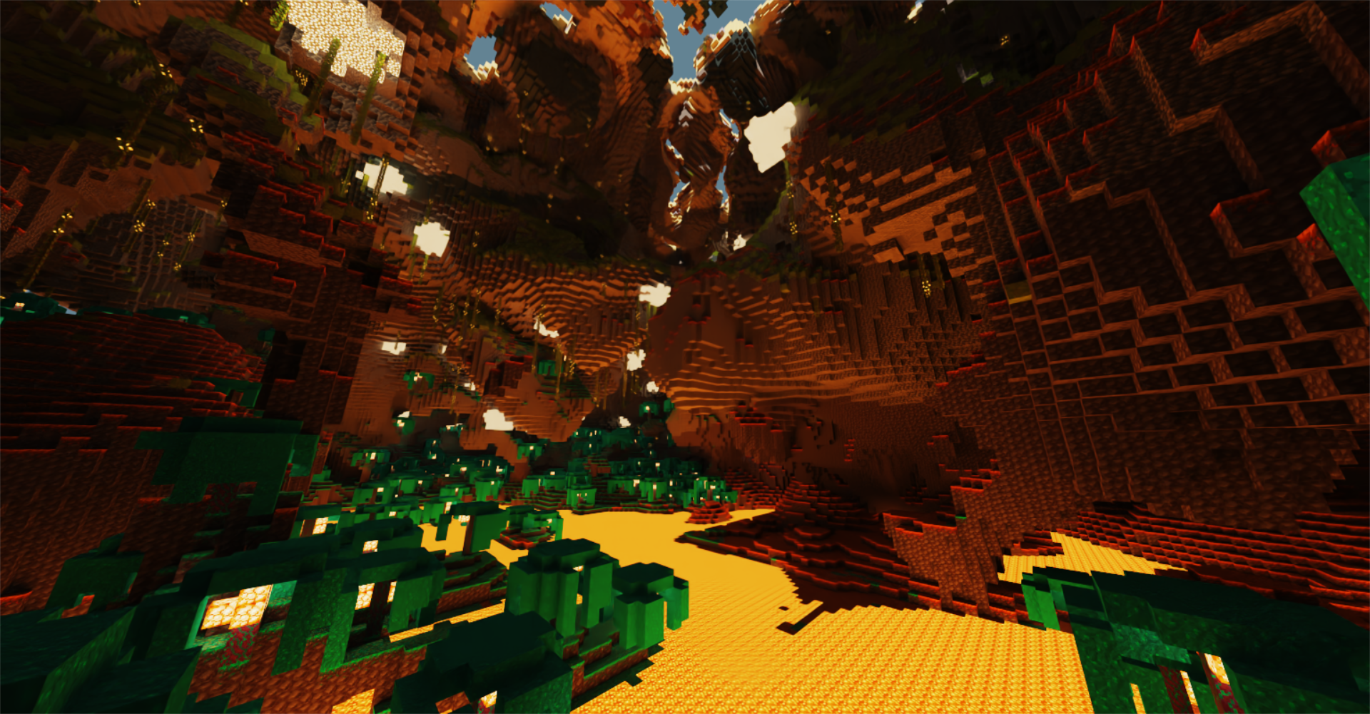
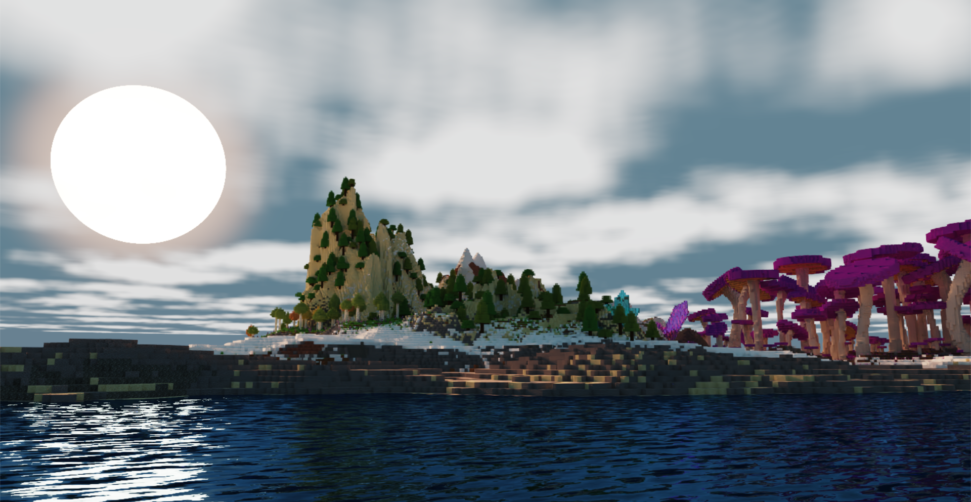
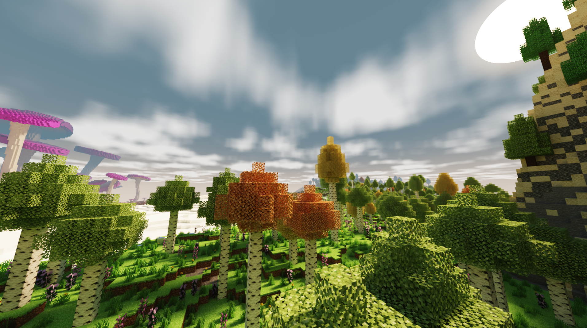
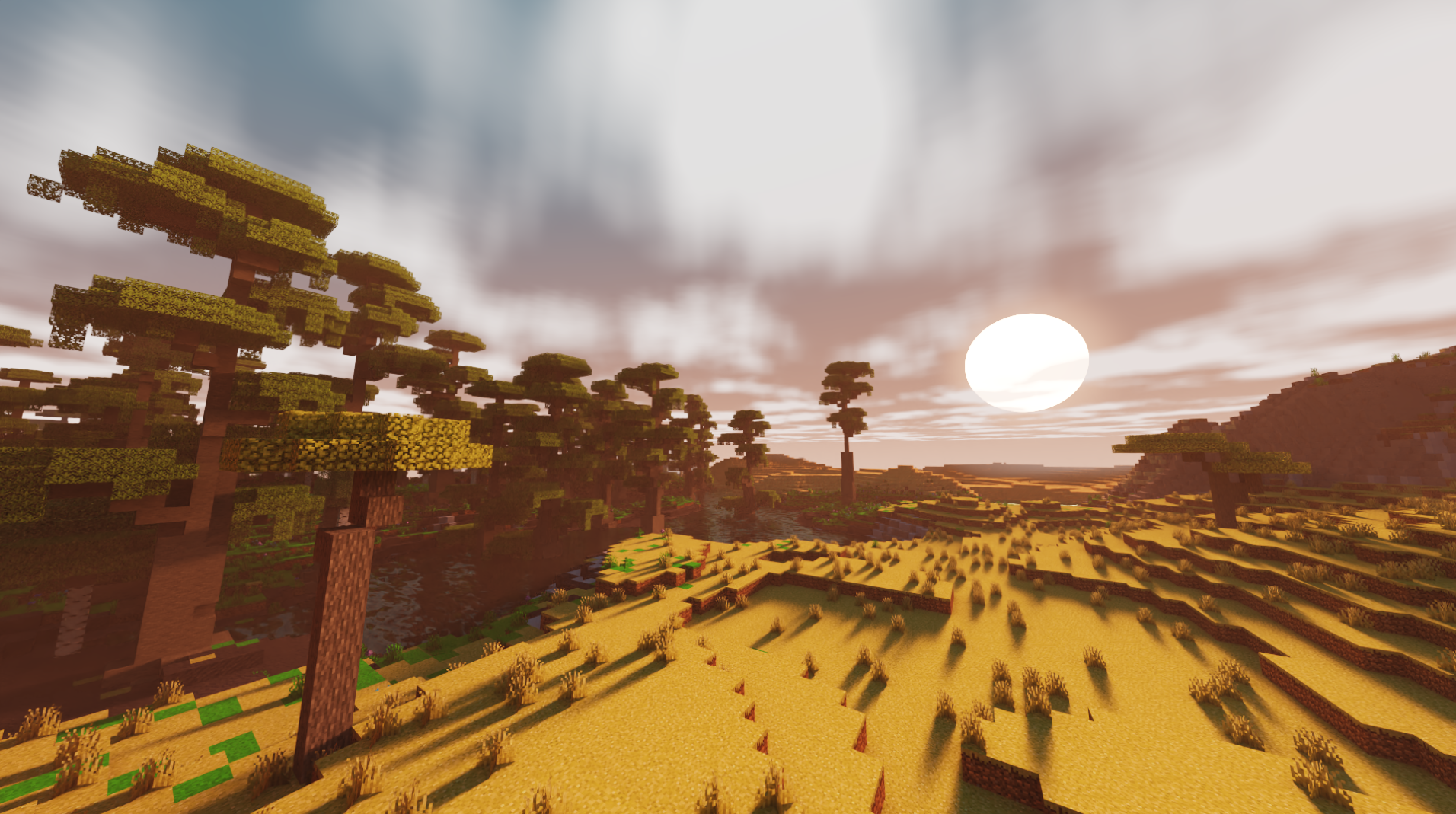
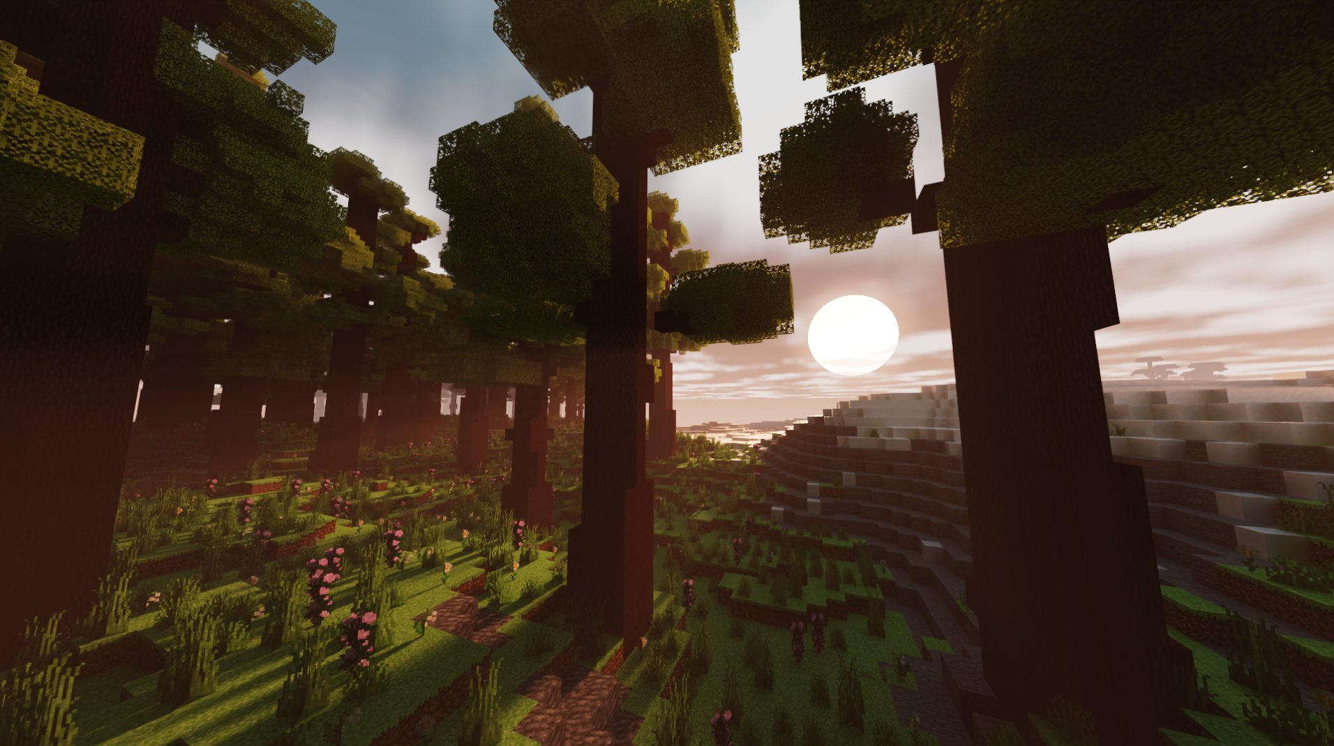
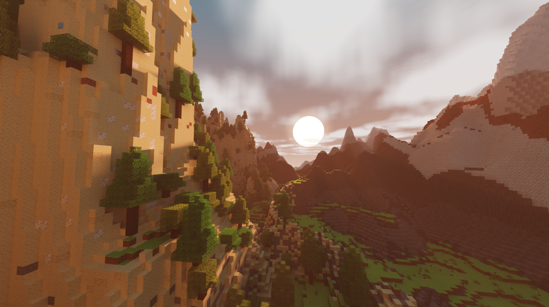
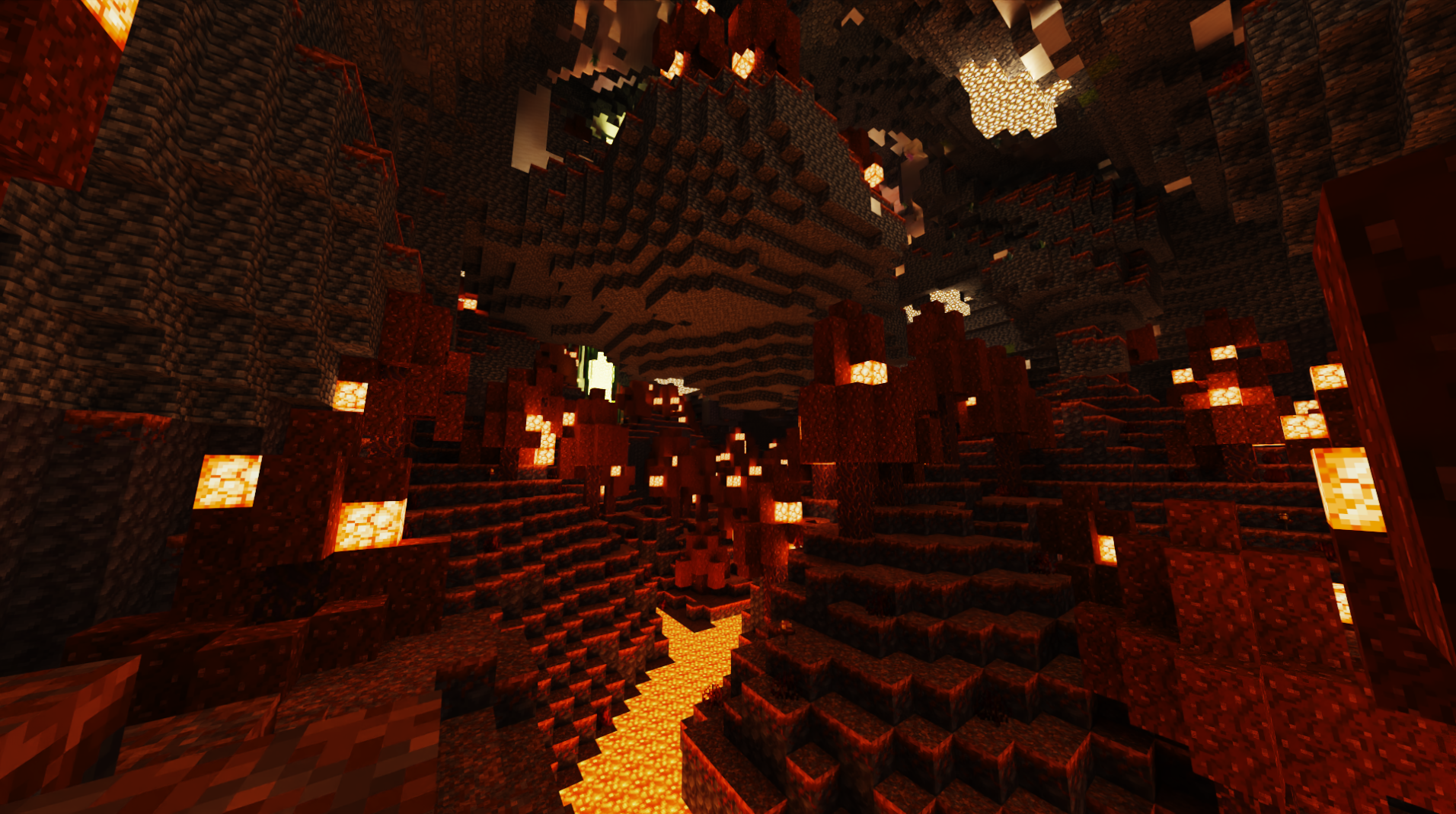
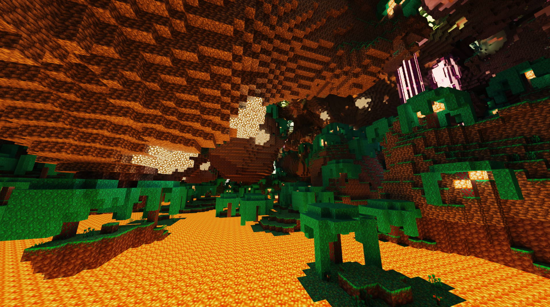
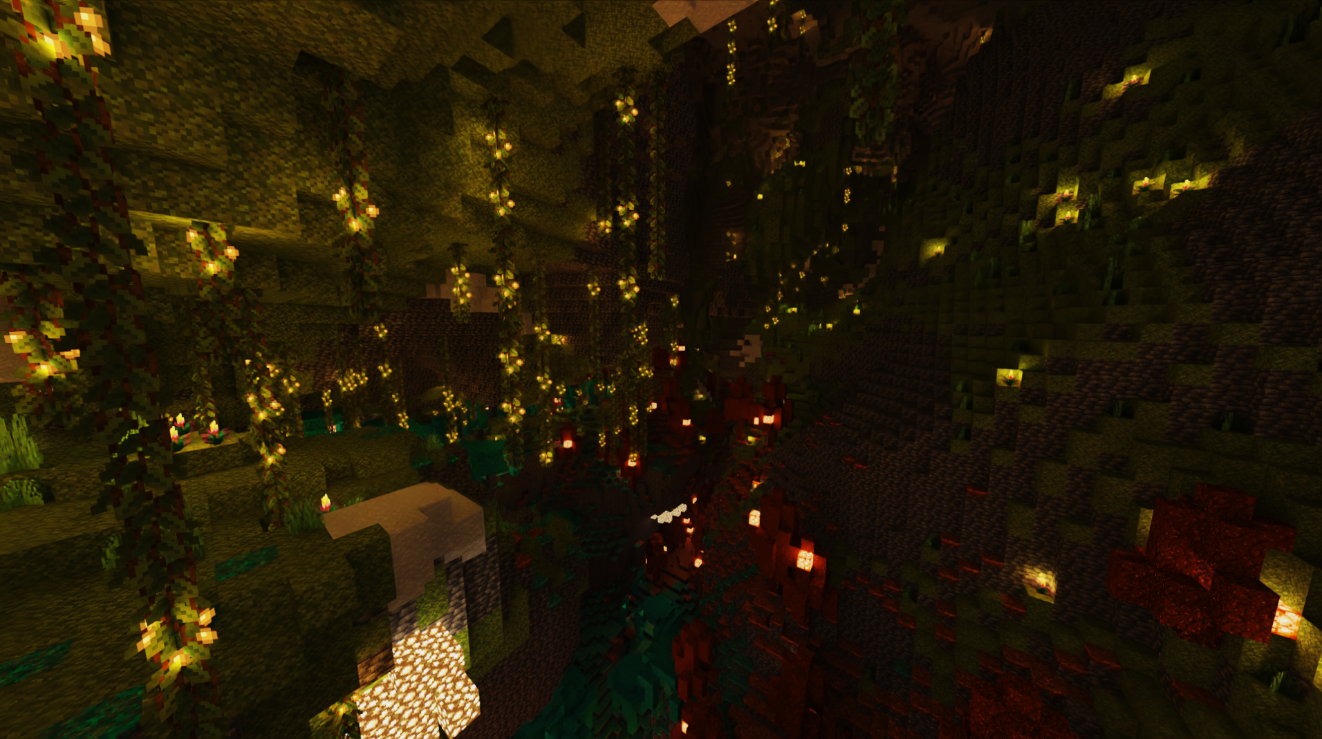
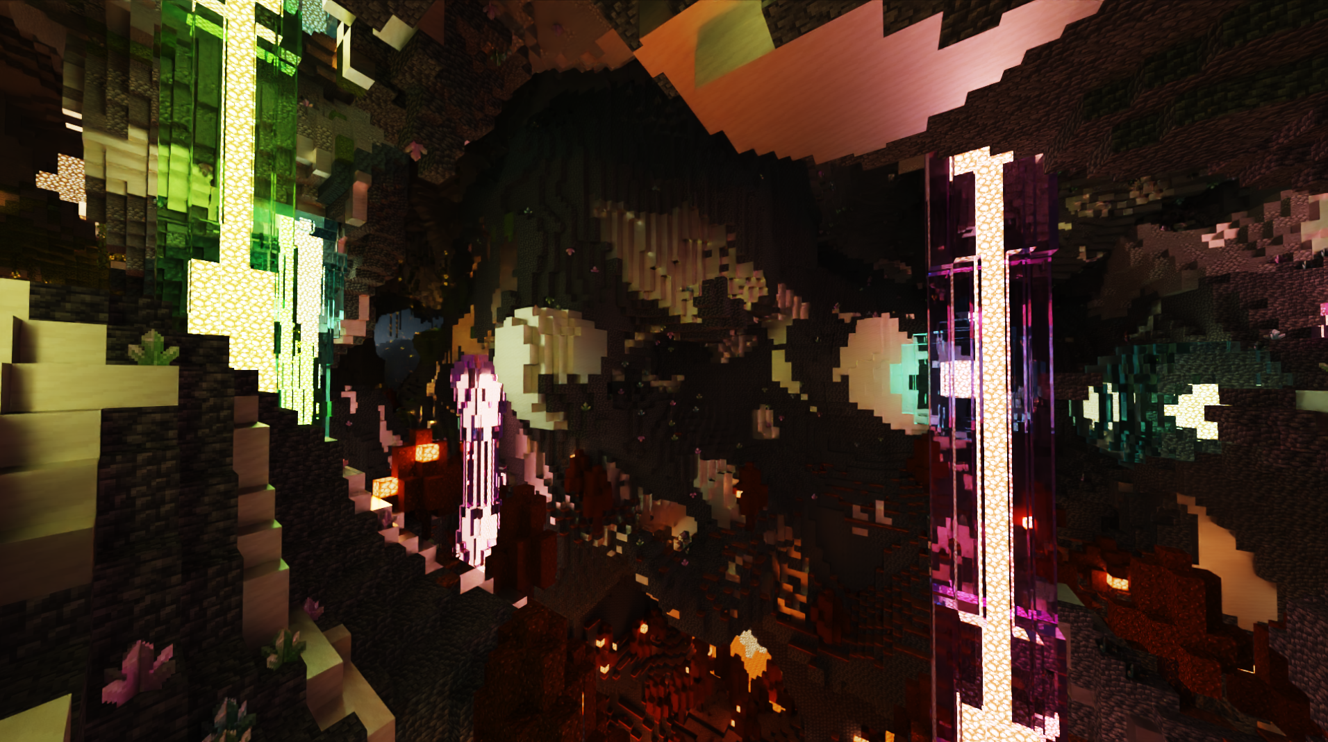
This project aims to recreate Minecraft with two major upgrades: real-time path tracing with OptiX and GPU-accelerated terrain generation with CUDA.
Minecraft is rendered by rasterization and a block-based lighting system, which works very well for gameplay. Minecraft shaders take that to the next level by introducing features such as shadow mapping, screen space reflections, and dynamic lighting. This project goes one step further by using the RTX accelerated OptiX framework to perform rendering entirely through path tracing, which gives realistic lighting, shadows, and reflections.
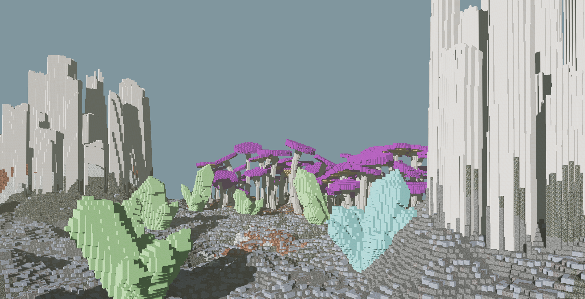
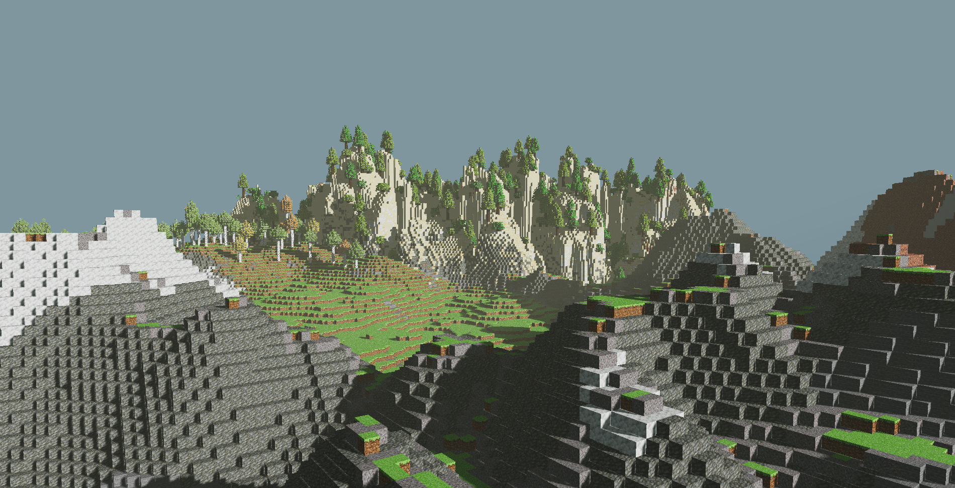
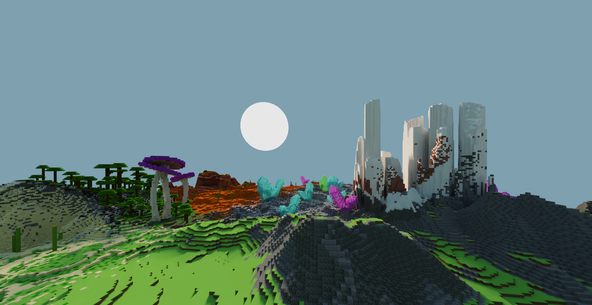
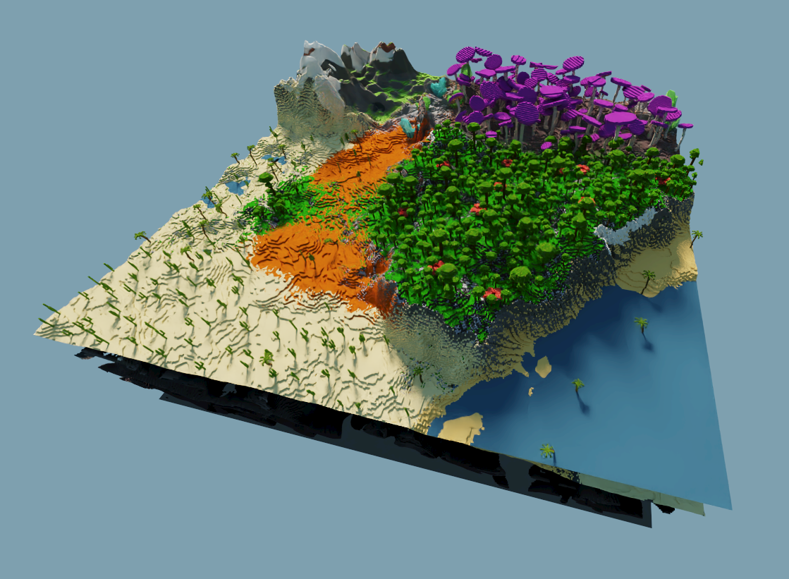
Additionally, GPGPU programming with CUDA allows for fast generation of fantastical terrain constructed from various noise functions and implicit surfaces. This project's terrain consists of several distinct biomes, each with their own characteristics and structures. Players exploring the world can find sights such as giant purple mushrooms, vast expanses of sand dunes, infected underground forests, and many more.
This README gives an overview of the various parts of the project as well as more detailed explanations of individual features.
When you run the project, there are a number of controls at your disposal.
WASDfor horizontal movementQto fly down,Eorspaceto fly up- Mouse to look around
LShiftto fly fasterZto toggle arrow key controls, which replace the mouse for looking around- Hold
Cto zoom in Pto pause/unpause time[and]to step backwards and forwards in timeFto toggle free cam mode, which disables generation of new chunks and unloading of far chunks
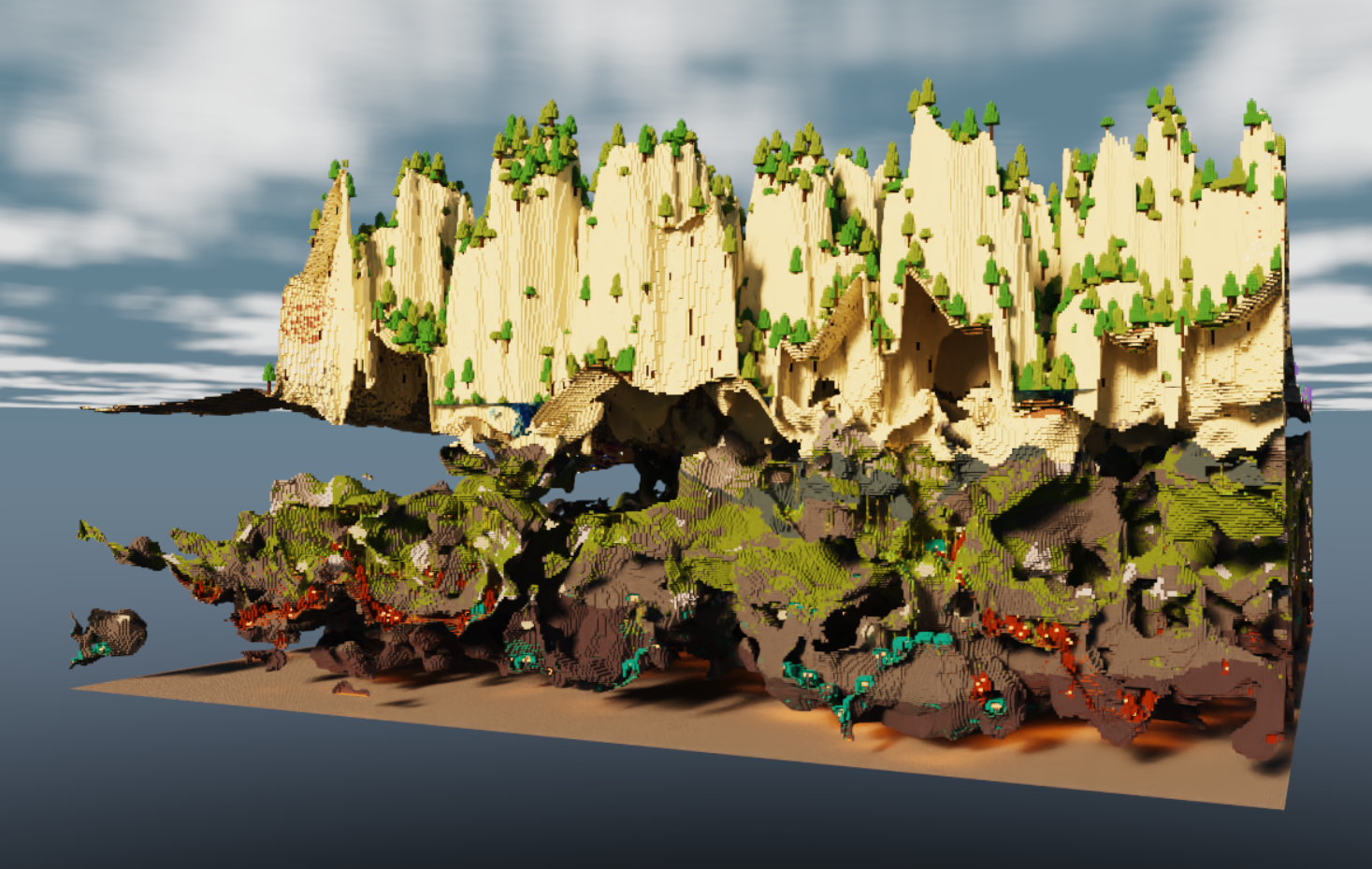
While an infinite procedural world is one of Minecraft's selling points, terrain has to be generated in discrete sections called "chunks". In normal Minecraft and in this project, a chunk consists of 16x384x16 blocks. As the player moves around the world, new chunks are generated while old chunks are removed from view.
Chunk generation in this project consists of several steps:
- Heightfields and surface biomes
- Terrain layers and erosion
- Caves and cave biomes
- Terrain feature placement
- This includes trees, mushrooms, crystals, etc.
- Chunk fill
Some steps, such as heightfields and surface biomes, can be performed on single chunks without any information about neighboring chunks. However, some steps, such as terrain layers and erosion, require gathering information from neighboring chunks in order to prevent discontinuities along chunk borders. The following dropdown sections explain the requirements for each step:
Heightfields and surface biomes
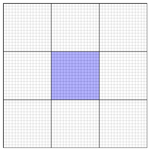
Generating heightfields and surface biomes considers only a single 16x16 chunk (blue).
Terrain layers
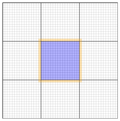
Generating terrain layers requires gathering some padding data (orange) from surrounding chunks to calculate the slope of this chunk's heightfield (blue).
Erosion
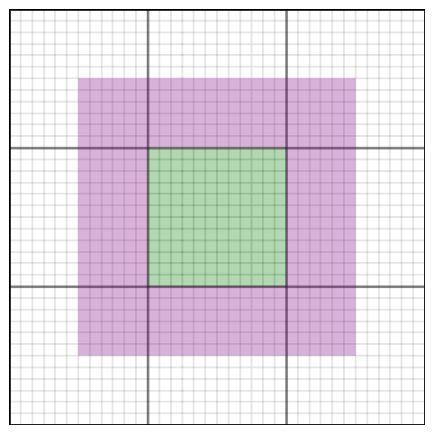
Erosion considers a 12x12 zone of chunks (green) with 6 chunks of padding on each side (purple).
Caves and cave biomes

Like for heightfields and surface biomes, generating caves and cave biomes considers only a single chunk (blue).
Terrain feature placement
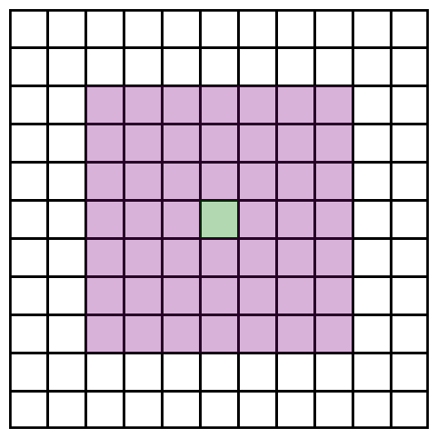
For generating terrain features, each chunk considers itself (green) and all chunks up to 3 chunks away (purple).
Chunk fill

Once all data has been gathered, this step fills an entire chunk (blue) with one kernel call.
To balance the load over time and prevent lag spikes, we use an "action time" system for scheduling. Every frame, the terrain generator gains action time proportional to the time since the last frame. Action time per frame is capped at a certain amount to ensure that no one frame does too much work. Each action has an associated cost, determined by empirical measurements of the step's average duration, which subtracts from the accumulated action time. For example, we currently accumulate up to 30,000 action time per second and allow up to 500 action time per frame. Generating a chunk's heightfield and surface biomes is relatively inexpensive, so its cost is only 3 per chunk. However, erosion is run over a 24x24 area of chunks at once and is relatively expensive, so its cost is a full 500 per 24x24 area.
Unless otherwise specified, all terrain generation steps other than gathering data from neighboring chunks are performed on the GPU using CUDA kernels. Additionally, we combined small kernels into mega-kernels to reduce launch overhead. For example, if we want to generate 100 chunks' heightfields, rather than launching one kernel for each one, we combine all the data into one long section of memory and launch a single kernel to do all the processing. This, combined with CUDA streams and asynchronous launches, allows us to generate terrain at a remarkably fast pace.
Lastly, we actually generate more terrain than is visible to the user at any given time. This extra padding not only ensures that large gathering steps (e.g. terrain erosion) don't get stuck where the player can see them, which would result in missing sections of terrain. Additionally, prebuilding far chunks allows for smooth loading of chunks as a player moves across the terrain.
The first step for a chunk is generating heightfields and surface biomes. Surface biomes consider only X and Z position, while cave biomes (discussed later) also take Y into account. All biomes are placed depending on multiple attributes, such as moisture, temperature, and rockiness, which are decided using noise functions. For example, the jungle surface biome corresponds to columns of terrain that are not ocean or beach, are hot, moist, and magical, and are not rocky. These noise functions also allow for smooth interpolation between biomes, such that the weights of all surface biomes and the weights of all cave biomes each add up to 1. Since each column's biomes and height are independent of all other columns, this process lends itself very well to GPU parallelization.
Biomes determine not only which blocks are placed, but also the terrain's height and which terrain features are created. For example, while the redwood forest biome has grass and redwood trees, the rocky beach biome has gravel and no notable terrain features. Both biomes also have relatively similar heightfields. These characteristics are blended in boundary areas using each biome's respective weight.
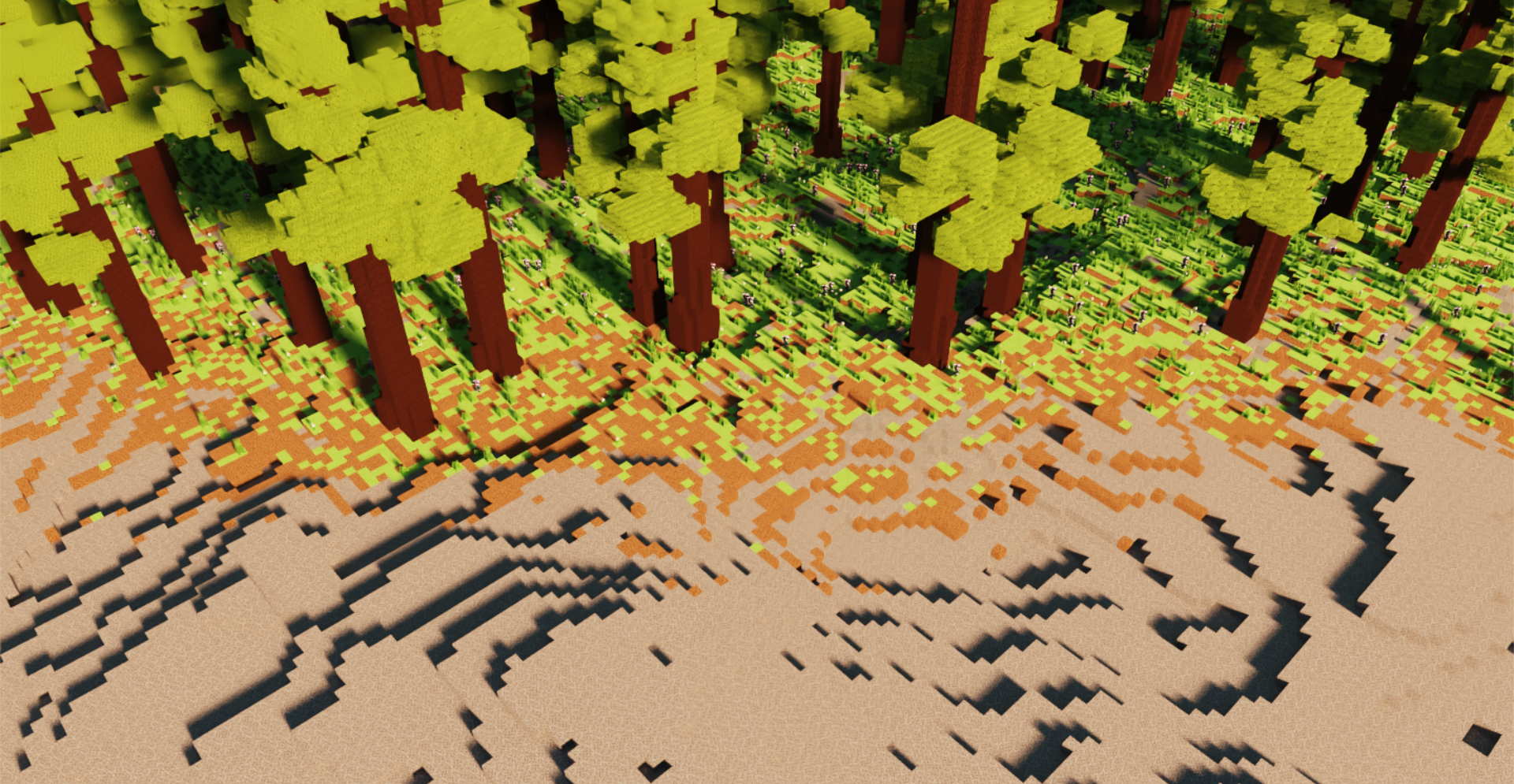
As the two biomes blend, their blocks also mix.
The height and biome weights of each column are stored for later use.
After heights and surface biomes are decided, the next step is to generate terrain layers and perform an erosion simulation. Our technique is based on Procedural Generation of Volumetric Data for Terrain (Machado 2019). First, layers of various materials (stone, dirt, sand, etc.) are generated using fBm noise functions. Each layer has parameters for base height and variation, and different biomes can also assign more or less weight to different layers. Layer heights are also smoothly interpolated between surface biomes based on the biomes' weights.
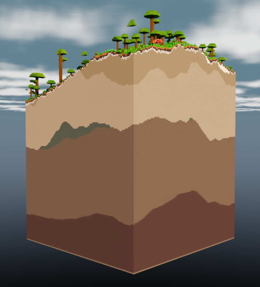
A section of 9x9 chunks showing various layers.
The top layers are "loose" and consist of materials like dirt, sand, and gravel. Loose layers' heights are determined in part by the terrain's slope, which requires gathering the 8 surrounding chunks of each chunk in order to determine the slope of the chunk's edges. Once all layers are placed, erosion proceeds starting from the lowest loose layer and going up to the highest. Rather than a traditional erosion simulation, which moves material from a column to its surrounding columns, we use Machado's proposed "slope method", which removes material from a column if it has too high of a difference in layer heights from its surrounding columns.
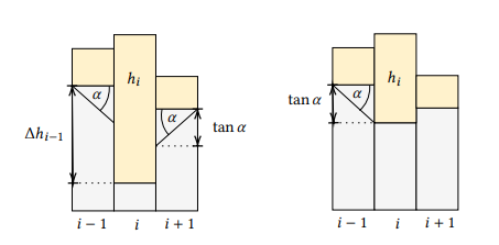
Illustration from the paper of the slope method, where α is the maximum angle between neighboring layers (defined per material).
The process is repeated until the terrain no longer changes. However, since erosion of a specified area relies on surrounding terrain data as well, performing this process on a chunk-by-chunk basis would lead to discontinuities. For that reason, we gather an entire 12x12 "zone" of chunks, as well as a further 6 chunks of padding on each side, before performing erosion on the entire 24x24 chunk area. Afterwards, we keep the eroded data for the center zone while discarding that of the padding chunks.
Erosion leads to more natural looking terrain, especially in steep areas. For example, in the jungle biome, erosion exposes subterranean stone in hilly areas while mostly ignoring relatively flat areas.
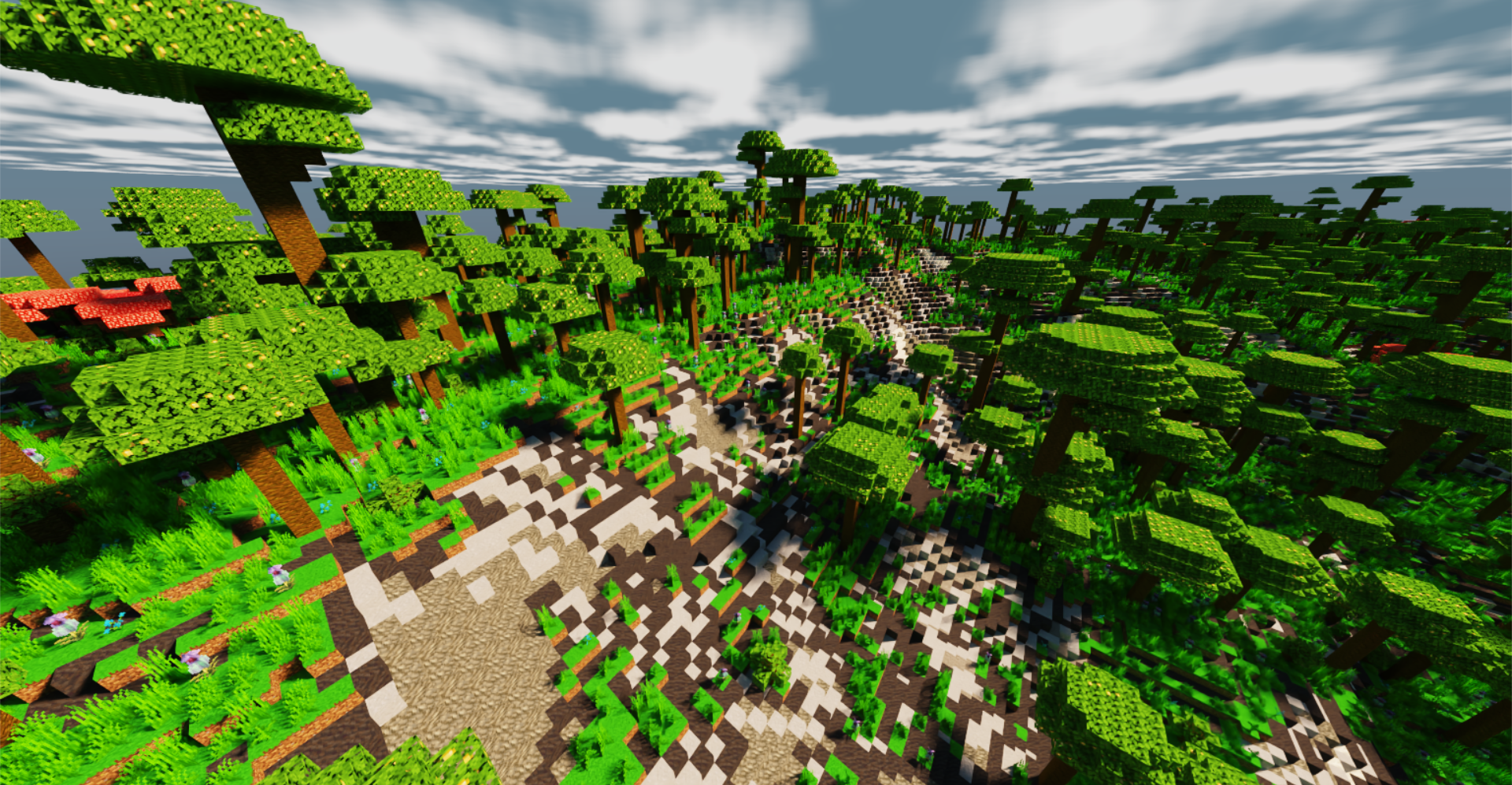
Notice how the relatively flat left side is mostly grassy while the steeper right side has much more exposed stone.
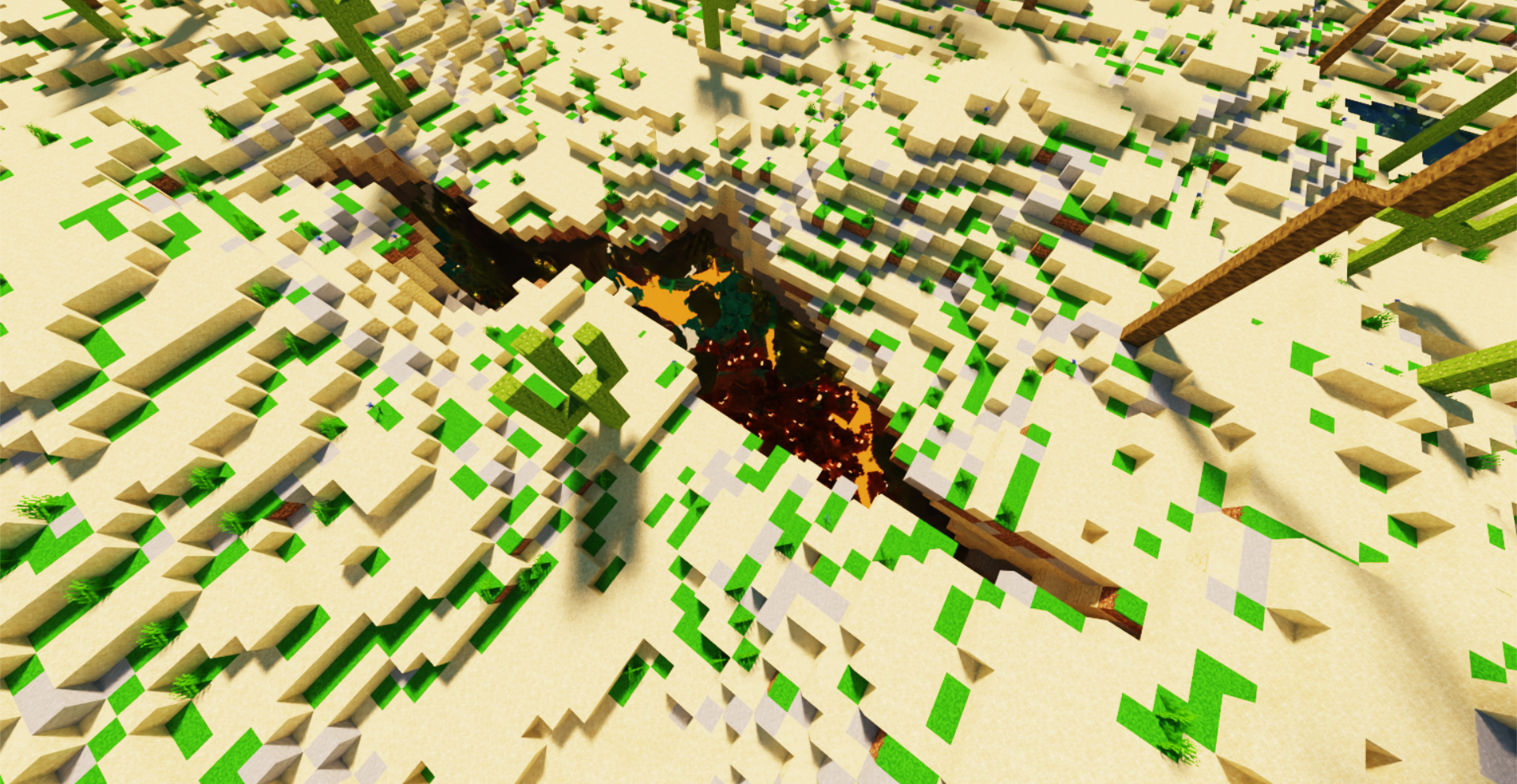
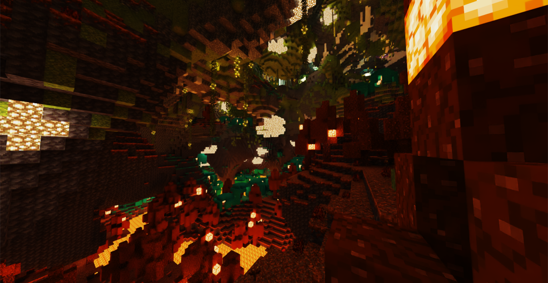
Once terrain erosion has completed, caves are carved out of the terrain. The main caves are heavily inspired by a Minecraft mod called Worley's Caves. True to their name, these caves use a modified version of Worley noise to generate infinite branching tunnels and large open areas. Most of the caves are hidden fully underground, but ravines located throughout the terrain provide access to the subterranean world.
The cave generation kernel first determines whether each block is in a cave, then it flattens that information into "cave layers". A cave layer describes a contiguous vertical section of air in a single terrain column. Each layer has a start and an end, as well as a start cave biome and an end cave biome. Cave biomes are determined in a similar fashion to surface biomes, except some cave biome attributes also take Y position into account. Each cave layer's biome is chosen at random, with each biome's weight serving as its chance of being chosen.
Flattening the 3D information into layers allows for easily querying the start, end, height, and biomes of any layer, which is essential for placing cave features (described in the next section).
At this point, the surface height, each cave layer's start and end height, and all biomes have been decided. The next step is to place terrain features, which is done on the CPU due to the inability to predetermine how many features a chunk will contain.
Each feature type has its own uniform grid with varying cell size and cell padding. For example, large purple mushrooms have a cell size of 10 and a padding of 2, meaning that each mushroom is placed at a random point in the center 6x6 area of a 10x10 grid cell. Each cell also has a certain chance of actually containing the feature, which helps give a more random appearance to the placements. For large purple mushrooms, the chance is 50%.
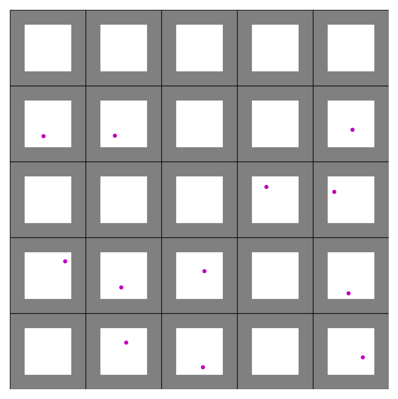
Continuing the purple mushrooms example, each grid cell (outlined by black borders) represents 10x10 blocks. Gray areas are padding and purple dots are feature placements.
Feature generators also contain lists of acceptable top layers so that, for example, trees are not placed on stone. For purple mushrooms, the only acceptable top layer is dirt at a thickness of at least 0.3. Even though the final top block in the biome is mycelium, the actual terrain layer is dirt and the mycelium is placed in the postprocessing step, meaning mushrooms will end up being placed on mycelium.
Each biome has its own set of feature generators. To place surface features, for each column of terrain, we first pick a random surface biome at random based on that column's biome weights. Then, for each of that biome's feature generators, we check whether any of them would generate a feature at exactly the current column's position, and if so, we place the feature on the current column with the chance set by the feature generation. Cave features are placed in a similar manner, except some of them generate from the ceiling as well. Cave feature generation uses the randomly predetermined cave biome of each cave layer instead of calculating a new random cave biome.
Since features can cross chunk boundaries, the last step is to gather the features of this chunk and surrounding chunks into one list to send to the final chunk fill kernel. Currently, the radius is set to 3 chunks, so features should be no more than 48 blocks wide.
The only thing left now is to actually fill the chunk's blocks. This step takes in various inputs:
- Heightfield
- Biome weights
- Terrain layers
- Cave layers
- Feature placements
If a position is below its column's height, it is filled in with a block depending on its corresponding terrain layer. If the block is in a cave layer, it will instead be filled with air. After the layers are filled out, some biomes also apply special post-processing functions. For example, the frozen wasteland biome turns water into ice while the mesa biome places layers of colorful terracotta. As with all other biome-related processes, these too are interpolated across biome boundaries using biome weights.
After the base terrain has been constructed, terrain features are filled in. Each thread loops over all gathered features and places the first one found at the current position. Feature placement generally consists of constructing implicit surfaces (e.g. signed distance functions) and checking whether the current position lies inside any of them. These surfaces range from spheres to hexagonal prisms to splines, and many are distorted by noise and randomness to give a more natural feel. For example, each purple mushroom consists of a spline for its stem and a cylinder for its cap. Additionally, the spline is actually made up of multiple cylinders at a high enough resolution to give a smooth appearance. Much of this logic was inspired by the approach of the Minecraft mod BetterEnd, which uses signed distance functions for its terrain features.
Feature placement also makes use of many early exit conditions to ensure that a thread does not perform intensive calculations for features which are nowhere near its position. Each feature type also comes with height bounds, which specify the upper and lower bounds of the feature type when compared to its placement point. This allows for determining the minimum and maximum height of all gathered features in a chunk, which in turn lets many threads safely exit without considering any feature placements.
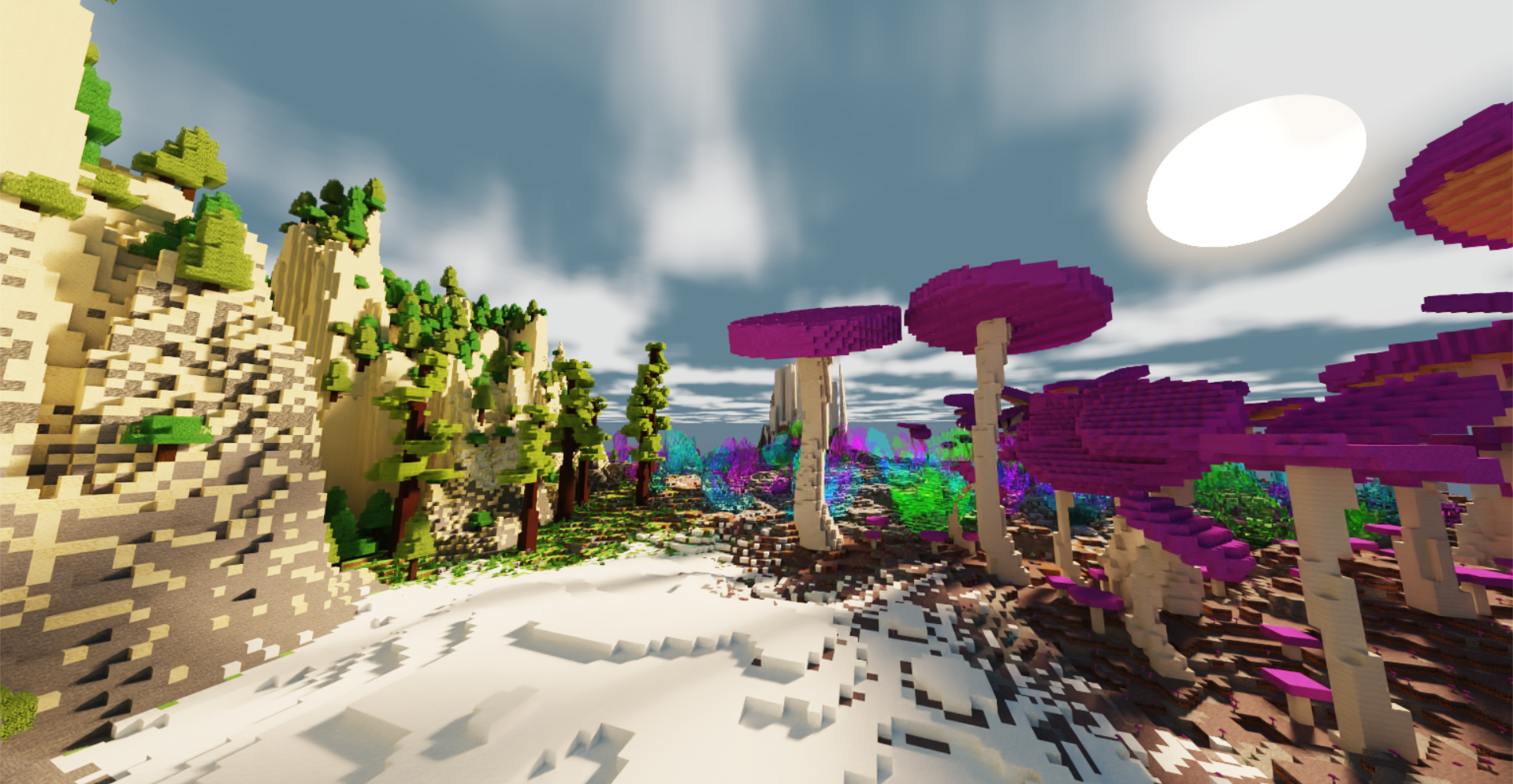
Various features placed across multiple different biomes.
Once all features are placed, the blocks are copied from the GPU to the CPU. Then, the last step is placing "decorators", which are blocks like flowers and small mushrooms. This is done on the CPU due to the potentially different number of positions to check for decorator placement in each column. Each biome has a set of decorator generators, each containing a chance per block, allowed bottom blocks (e.g. grass for flowers), allowed blocks to replace (usually air but can be water for ocean decorators), and optionally a second block for decorators that are two blocks tall. Some decorators, like crystals in the crystal caves, can even generate hanging from the ceiling.
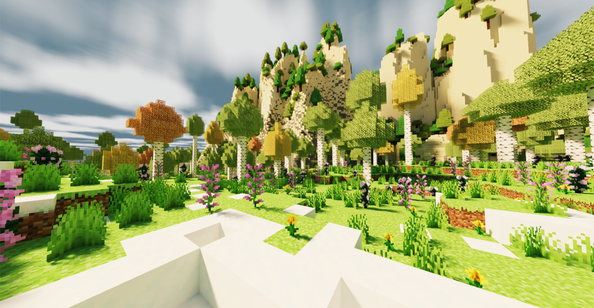
Decorators in the lush birch forest biome, including grass, dandelions, peonies, and lilacs.
Once decorators are placed, the chunk's block data is fully complete. All that remains is creating vertices from the blocks and sending those to the GPU to construct acceleration structures.
To efficiently and realistically render the terrain, this project uses hardware-accelerated path tracing which supports [list features here]. The path tracer itself is built with NVIDIA OptiX 8.0, while the final frame rasterizer and game window use DirectX 11 and the Windows API.
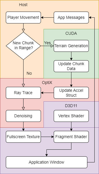
Flowchart outlining application process and API segmentation.
As shown in the flowchart above, each frame starts from processing any application messages. If an application message is received, it triggers a corresponding scene state update, which may be a player movement, window resize, zoom adjustment, or camera rotation. All of these events can cause changes in the currently visible region, which triggers the terrain generation process for newly visible chunks and unloads chunks that are too far. Once chunk generation is complete, it causes an update to the acceleration structures used by the path tracer. Regardless of whether new chunks are generated, the path tracing procedure is then launched to actually render the scene. The noisy output from path tracing, along with albedo and normals guide images, are then denoised. The final denoised output is then transferred to DirectX 11, which renders the frame using a single triangle that covers the entire screen.
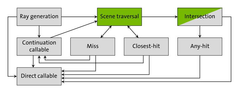
The path tracer consists of various OptiX programs, which are similar to regular shaders in that they are located on the GPU and represent different shading operations. They are also organized into different program groups that represent different functionalities. All shader program groups are stored in a Shader Binding Table (SBT).
Dispatching an OptiX render will first call the raygen program group. This program group not only determines which pixel a thread corresponds to and generates a ray pointing at that pixel, but it also iterates through the ray's bounces and even launches occlusion rays for shadow calculations.
Then, the hit program groups are called when a ray hits geometry in the scene. There are two types of hit programs: any-hit and closest-hit. Any-hit programs are called on any intersection; we use them to ignore intersections with full transparency (e.g. in tall grass and flowers). Closest-hit programs are called on the closest intersection; these are where we evaluate BRDFs, accumulate light, and determine how rays bounce.
If a ray does not hit any geometry, it instead calls a miss program group. In our project, miss program groups are used mostly for occlusion testing and sky shading.
Lastly, buffering the scene geometry to the GPU requires further setup. As the user navigates through the terrain, new chunks are generated while old chunks are unloaded. To allow for this dynamic rendering of chunks, we use a two-layer setup of acceleration structures. Each chunk is represented by a Geometry Acceleration Structure (GAS), which are children of a top-level Instance Acceleration Structure (IAS). This allows for easily adding and removing chunks (GASes) from the current set of geometry, as the device-side handle of the IAS never changes.
Combining the OptiX programs and acceleration structures results in a full path tracing pipeline:
The OptiX path tracer uses several physically based shading techniques to shade the terrain in a realistic manner. Due to the complexity of the terrain with various emissive objects, an accurate light simulation is necessary to correctly simulate the light interaction at any location in the scene. The path tracer achieves this with global illumination; this technique multiplies the intersection's color with the color of the ray and adds this color accumulation to the pixel associated with the ray's initial direction. As a ray bounces through the scene, the pixel represented by the ray accumulates the colors from all the ray intersections, lights, and the sky.
Additionally, the path tracer uses direct lighting to add light influence on a ray's pixel when a light source (the sun) is visible from the ray's intersection point and is not occluded by any geometry. This technique adds strong, visible shadows that converge much faster than they would through just random hemisphere sampling. Soft shadows can also be simulated by sampling the entire surface of a light source, such as the circular area covered by the sun. Since direct lighting cares only about whether it hits anything and not what the closest hit is, it uses a different ray type than normal path tracing to more efficiently check for intersections without any unnecessary steps.
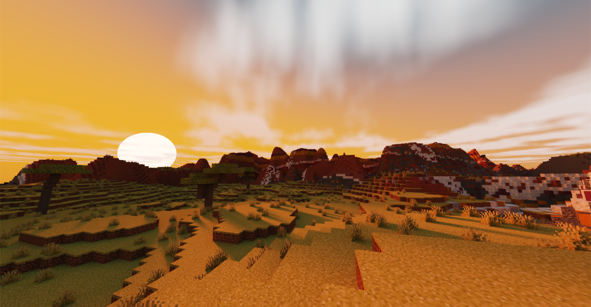
Objects block sunlight and cast shadows on surfaces.
Different materials in the scene also reflect light differently. Most notably, water and crystals exhibit specular reflection and refraction. When a ray hits that type of geometry, the ray either reflects away from the surface or refracts into the surface based on random chance determined by the materials' index of refraction. Some other materials with reflective properties, such as sand and gravel, have microfacet roughness reflectivity that makes them appear slightly reflective without being transparent.
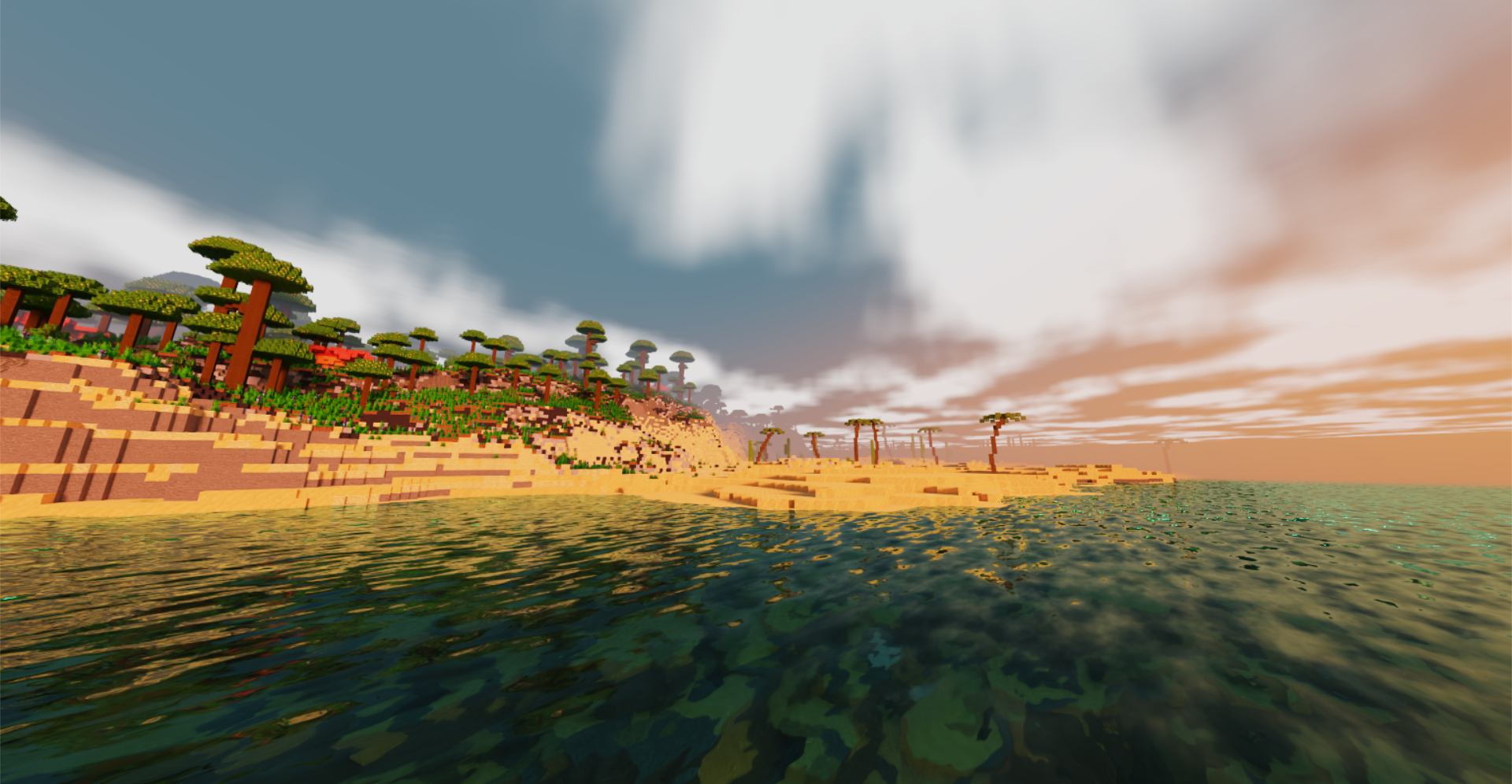
Water is reflective and also see-through.
Finally, rays may experience volumetric scattering in the scene during certain times of day, most notably at dawn and dusk. If a ray is scattered, it does not reach its intended destination and instead bounces around a volume. However, it is inefficient to simulate multiple cases of scattering of a ray in a random direction, especially in real-time applications, so the path tracer checks for direct lighting at a ray's first scattering occurrence. If the scattered ray is not directly illuminated by a light source, the ray is considered "absorbed" by the volumetric particle. This technique creates volumetric fog, which is best represented by light rays traveling through gaps in the terrain.
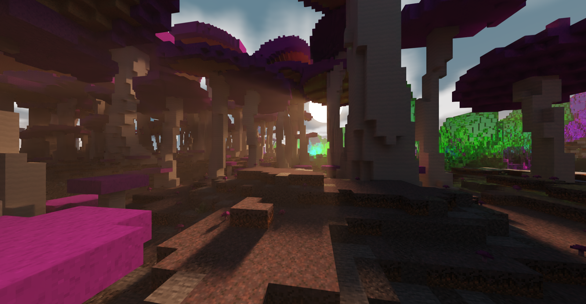
Rays of sunlight going through gaps between mushroom stems.
We made various optimizations to our OptiX pipeline to improve path tracing performance. Special thanks goes to Detlef Roettger for advising us on this topic.
First, we choose debug logging and error checking levels based on whether we are launching the project in debug or release mode. Debug messages provide invaluable information for solving issues with the project, but enabling them can severely degrade performance. In release mode, we remove most logging and error checking to allow for much higher performance.
Next, since the maximum number of renderable chunks at once is known ahead of time as a function of the maximum render distance, we can preallocate memory for certain structs to avoid having to allocate memory on the fly. We also store an array of chunk data with a fixed maximum size along with a pool of chunk IDs that is drawn from whenever a new chunk is created. These methods allow for easily updating GASes and the IAS each frame if necessary. The structure of the GASes and IAS is also important; we use the previously mentioned hierarchy with many GASes under one IAS along with the scene hierarchy flag OPTIX_TRAVERSABLE_GRAPH_FLAG_ALLOW_SINGLE_LEVEL_INSTANCING to take full advantage of RTX cores.
Additionally, each frame's final denoised output is rendered directly into a D3D11 texture using CUDA-D3D11 interop, which removes the need for costly transfers between host and device. The D3D11 renderer itself uses an oversized fullscreen triangle to render to the screen, which avoids the possible redraws that can come with a fullscreen quad. The vertex shader also generates vertex positions and UVs directly to minimize its memory footprint.
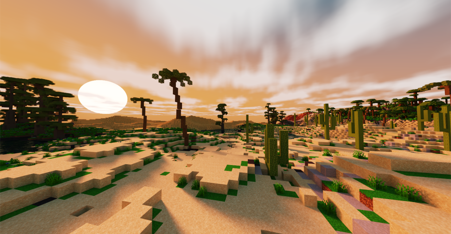
The sky includes a full day and night cycle, complete with a sun, moon, clouds, and stars. During sunrise and sunset, the sky becomes a bright orange near the sun. Additionally, since they are the main sources of light on the surface, the sun and moon are also sampled for direct lighting to reduce noise.
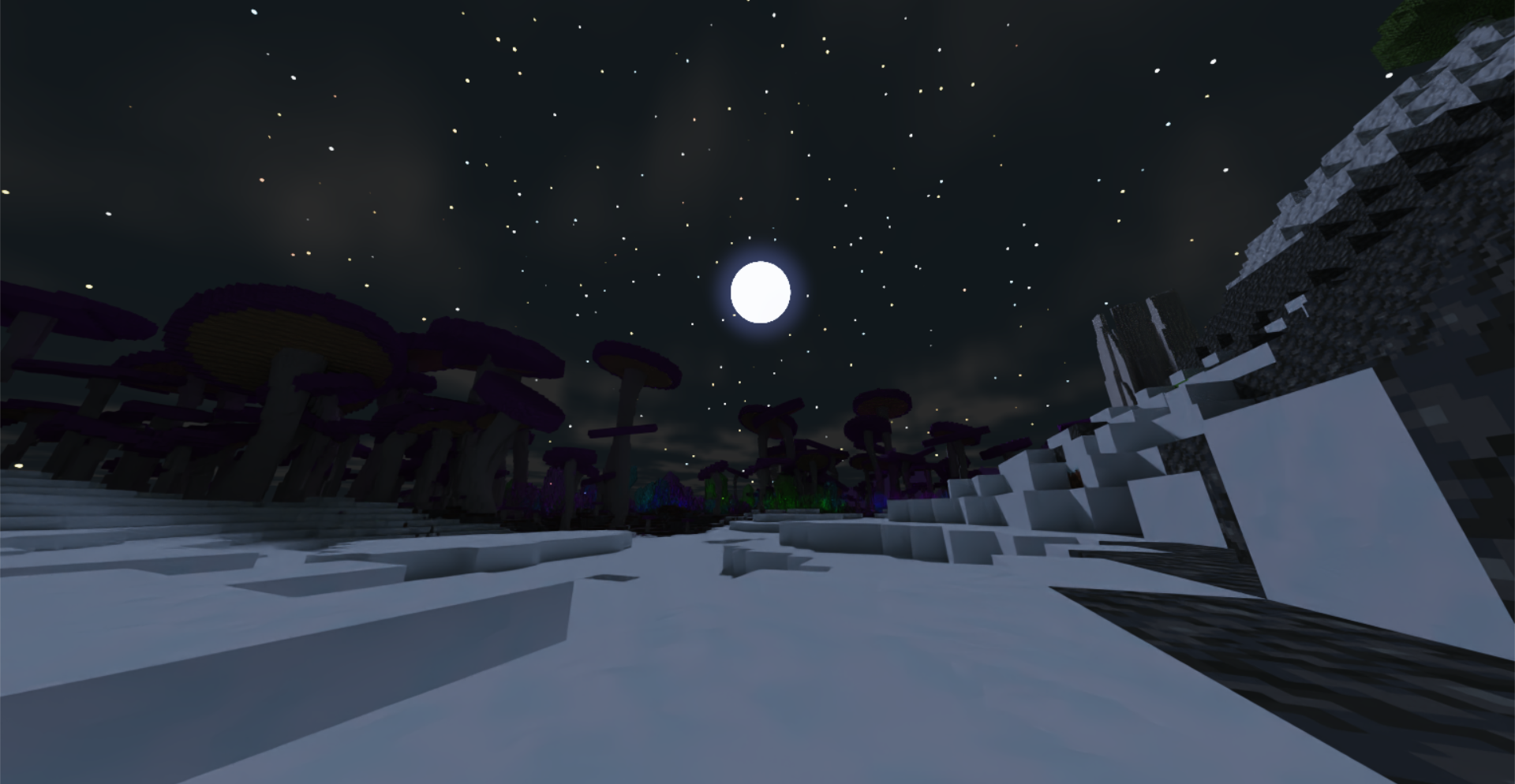
Shadowy fungi against a starry night sky.
The denoiser implemented in this program is the AOV denoiser packaged with OptiX 8. The denoiser can optionally be set to 2x upscaling mode, which renders at half the preset render resolution and uses the denoiser to upscale back to the original size, reducing the raytracing workload. This section gives a brief overview of each denoiser and its pros and cons. For more details on the denoisers, please refer to the official API documentation linked below in the references section.
The AOV denoiser takes in a noisy path traced image as well as auxiliary albedo and normals buffers. it also does some additional calculations for HDR inputs to determine the average color. Then, using a pre-trained neural network, it outputs a denoised final image. Using the auxiliary buffers greatly increases the denoiser's efficacy, especially in areas without much direct lighting, as the denoiser can more easily distinguish between different blocks and colors.
Using a denoiser does result in a noticeable performance drop, but it leads to much faster convergence of the final image. It takes less than a second for the render to fully converge when aboveground. When underground, it takes around 5 seconds since we do not sample emissive surfaces for direct lighting.
One caveat of the denoiser is that it does not work very well when the player is in motion. There is noticeable camera flickering as the path tracing noise moves across the screen, and the problem is once again exacerbated in caves due to the lack of direct lighting.
The 2x upscaling AOV denoiser acts very similarly to the regular AOV denoiser, except that it additionally scales the image up by 2x. This allows for keeping the final render size constant while halving the raytracing resolution, effectively reducing the raytracing workload to 25%.
This comes with the obvious advantage of greatly increasing performance. We saw around a 2x improvement in performance when rendering at 720x540 and 1920x1080. Additionally, this model can be used for "supersampling" by raytracing at the window resolution, scaling up to 2x using the denoiser, then downsampling to the window resolution.
However, this denoiser of course comes with some disadvantages. The main disadvantage is that areas with high frequency detail tend to become blurry. For example, tree leaves generally have high frequency detail because leaf textures have many transparent pixels mixed in among opaque pixels.
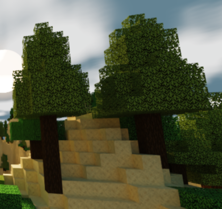
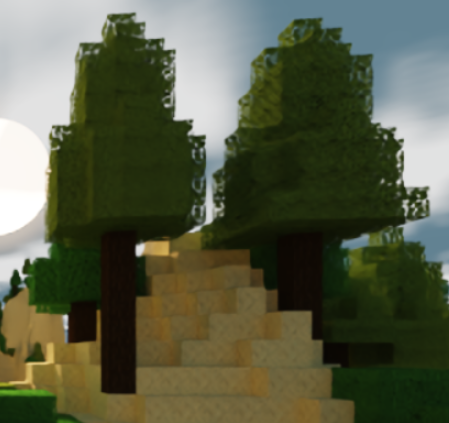
The same two trees, rendered at full resolution (left) and half resolution with upscaling (right). Notice that the leaves are much blurrier with upscaling.
Additionally, as with the regular AOV denoiser, this denoiser does not work very well with motion.
Sections are organized in chronological order.
- Procedural Generation of Volumetric Data for Terrain (Machado 2019)
- Physically Based Rendering: From Theory to Implementation
- Ingo Wald's OptiX 7 course
- OptiX Programming Guide and API documentation and OptiX Applications
- CUDA Programming Guide
- Worley's Caves
- BetterEnd
- Detlef Roettger for giving us invaluable OptiX advice and looking through our codebase
- Eric Haines for putting us in contact with Detlef
- Henrique Furtado Machado for discussing the details of his paper with us
- Wayne Wu, Shehzan Mohammed, and the TAs for teaching CIS 5650
- Adam Mally for assigning the original Mini Minecraft project
