AkiraKane/data-science-interview

Data Science Interview projects collections

Data Science Cheat Sheet

Useful Links

• OVER 100 Data Scientist Interview Questions and Answers!
• DS 面试 统计类问题 学习资料总结
• A/B testing 知识点整理

MySQL Cheat Sheet

Some refer links:

• SQLZOO

Basic

• Alias, every derived table must have its own alias. SELECT ... FROM (subquery) [AS] x. NOTE: don't use alias in WHERE clause.
• GROUP BY ... HAVING aggregate_func, NOTE WHERE clause is before GROUP BY.
• WHERE x = (SELECT MAX(...) FROM ...), NOTE: WHERE x = MAX(...) is wrong, aggregate function can't show in where clause.
• WHERE column = value, WHERE column in (subquery), WHERE (column1, column2) in (subquery).
• LIMIT m, n = LIMIT n OFFSET m, skip top m rows then top n rows.
• COUNT(...) & COUNT(DISTINCT ...), can use count distinct for multiple columns. Conditional count COUNT(IF (condition, 1, NULL)) or SUM(condition[x1 = x2]), conditional ratio AVG(condition).
• Round, ROUND(..., decimals).
• Union, combine records from multiple columns into one. UNION = UNION DISTINCT -> remove duplicates, UNION ALL -> keep duplicates.
• String, SUBSTRING(str, num1, num2), extract a substring from str (start at position num1, length num2).
• Condition Judgement, CASE WHEN <condition> THEN ... ELSE ... END, CASE <value> WHEN <value> THEN ... END, note there're two ways expressions. Some other condition judgement methodIF(..., value if True, value if False), IFNULL (value if not null, value if null). COALESCE(value1, value2) has same function with IFNULL, COALESCE is to choose the first not null value in list, so in application if value1 is null then value2 replaces it.
• Create, CREATE TABLE table_name (column_name1 column_type1, column_name2, column_type2, PRIMARY KEY (column_name1)).
• Insert, INSERT INTO table_name (field1, field2) VALUES (value11, value12), (value21, value22).
• Update, UPDATE table SET column = value [WHERE].
• Delete, DELETE FROM table [WHERE clause], an classic example.
  DROP > TRUNCATE > DELETE. DROP TABLE drop entire table, TRUNCATE TABLE delete all records of table, both can't revise. DELETE delete specific records, can revise.
• Like, fuzzy query for string. SELECT * FROM table WHERE column1 LIKE '%THIS, % stands for any 0 or multiple chars, _ stands for single chars, for other regular expression.
• Random, RAND(seed=None), returns a random number between [0, 1). Get random int between [0, 10], SELECT FLOOR (RAND() * 11).
• Index, index can boost query while need more space, which will slow down alter process(insert). INDEX could be duplicated and null. Primary Key will automatically generate UNIQUE INDEX(unique and not null).
• Explain, EXPLAIN query, check SQL query plan.

Date

• Date, DATE('2020-01-01') is a date type. Query date in one year or one month, YEAR(date) = 2020 or MONTH(date ) = 4. Change format of the date DATE_FORMAT(date, '%m-%d-%Y'), can use other format specifiers.
• DATE_ADD(date, INTERVAL number type[DAY, WEEK, MONTH, YEAR]), DATE_SUB(date, INTERVAL number type[DAY, WEEK , MONTH, YEAR]).
• DATEDIFF(date1, date2) = date1 - date2.
• CURRENT_DATE() = CURDATE() get current date. NOW() get current datetime.

Advanced

• View & CTE

  • View stores the query, it's just like a virtual table.
    1. Simplify frequent query operation.
    2. For security reason, can show limit data to specific users.
  • CTE is a temporary result set that exists only within single SQL statement, like subquery.
    1. CTE doesn't store as an object.
    2. CTE can be referred multiple times in the same query and used in recursive calculation.

• Median, there's no function to get Median in MySQL.

SELECT AVG(salary) as median 
FROM 
    (SELECT salary, ROW_NUMBER() OVER() AS row, COUNT() OVER() AS total_rows
     FROM table) AS x
WHERE row BETWEEN total_rows/2 AND total_rows/2+1

• Variable, SELECT @variable := <some change> FROM table1, (SELECT @variable := original value) AS X. NOTICE SPACE.
• Rank() OVER(PARTITION BY ... ORDER BY ...). ROW_NUMBER() makes ordinal rank without tie. DENSE_RANK() doesn't take gap for tie.
• Some useful window function. FIRST_VALUE() get first value, LEAD() get next value, LAG() get previous value.
• Window Function, Function() OVER(PARTITION BY ... ORDER BY ... ROWS [BETWEEN] <frame_start> [AND] <frame_end>).
  1. frame_start:
     1. UNBOUNDED PRECEDING: frame starts at the first row of the partition.
     2. N PRECEDING: a physical N of rows before the first current row. N can be a literal number or an expression that evaluates to a number.
     3. CURRENT ROW: the row of the current calculation.
  2. frame_end
     1. frame_start: as mentioned previously.
     2. UNBOUNDED FOLLOWING: the frame ends at the final row in the partition.
     3. N FOLLOWING: a physical N of rows after the current row.
• Create Function

DELIMITER $$

CREATE FUNCTION function_name(
    param1 datatype,
    param2 datatype,
    …
)
RETURNS datatype
[DETERMINISTIC]
BEGIN
 -- statements
END $$

DELIMITER ;

Python Algorithms Cheat Sheet

Data Structure & Standard Library

• collections

  • Counter. Dict subclass for counting hashable objects.
    • most_common(n: int = None), get TOP N frequent (elements, count) list of tuple.
  • defaultdict. Dict subclass that calls a factory function to supply missing values.
    • defaultdict(list)[key] = dict.setdefault(key, []), same for other data type: int, set.
  • deque. List-like container with fast appends and pops on either end. Tips: good choice for BFS.
    • append(x) & appendleft(x). Append one element to right & left side.
    • extend(l) & extendleft(l). Extend the iterable object (list) to right & left side. Note left one will be reversed.
    • pop() & popleft(). Pop out one element from right & left side.
    • count(x). Count the number of element x. reverse() & remove(x) are inplace methods same with List.
    • rotate(n=1). Rotate the deque n steps to the right. If n is negative, rotate to the left, rotating one step to the right is equivalent to d.appendleft(d.pop()), and rotating one step to the left is equivalent to d.append(d.popleft()).

• heapq. Heap is a binary tree like data structure, with all parent nodes value less(more) than or equal to its own children. Heapsort is O(nlogn) sorting algorithm. In python heaqp, default is min-heap, which the smallest is always the root, head[0].

  • heapify(x). Transform list x into a heap (still a list type), in-place, in linear time.
  • heappush(heap, item). Push the value item onto the heap, maintaining the heap invariant.
  • heappop(heap). Pop and return the smallest item from the heap, maintaining the heap invariant.To access the smallest item without popping it, use heap[0].
  • heappushpop(heap, item). Push item on the heap, then pop and return the smallest item from the heap.
  • heapreplace(heap, item). Pop and return the smallest item from the heap, then push the new item.
  • merge(*iterables, key=None, reverse=False). Merge multiple sorted inputs into a single sorted output.
  • nlargest(n, iterable, key=None). Return a list with the n largest elements from the iterable. Equivalent to sorted(iterable, key=key, reverse=True)[:n].
  • nsmallest(n, iterable, key=None). Return a list with the n smallest elements from the iterable.Equivalent to sorted(iterable, key=key)[:n].

• Trie. Trie aka prefix tree, is a kind of search tree for strings. For all children of one node share the same prefix, each node represents one letter and usually has 26 children. In Python, Trie need to be manually defined. Trie is constructed by TrieNode(two attributes children: Dict & end: bool). 208. Implement Trie (Prefix Tree)

  • __init__. Initialize with empty root node.
  • insert(String). Generate children of parent node recursively, if the letter key not in parent node then create one. In the final node, set end = True, meaning it's a completed word.
  • search(String). Search if the word in the trie.
  • word_suggest(String). Give out suggestion result when tying in a searching word. 1268. Search Suggestions System

• random. Generate pseudo-random numbers.

  • random(). Return random float number in [0.0, 1.0).
  • randrange(start, stop, step). Return a randomly selected element from range(start, stop, step).
  • choice(seq). Return a random element from the non-empty sequence.
  • sample(population, k). Return a k length list of unique elements randomly selected from population. Sampling without replacement.

• bisect. Support for maintaining a list in sorted order without having to sort the list after each insertion.

  • bisect(a, x, lo=0, hi=len(a)). Return an insertion index partition the sorted list a into two parts that left <= x < right. 981. Time Based Key-Value Store
  • bisect_left(a, x, lo=0, hi=len(a)). Similar with above. left < x <= right.
  • insort(a, x, lo=0, hi=len(a)). insort_left(a, x, lo=0, hi=len(a)). Insert x into sorted list a.

• copy. Compare assignment & shallow copy & deep copy. Link

Algorithm Summary

• DFS & BFS
  • DFS can reach the target, but might not take the optimal steps/route. Thus BFS is a good choice for optimal search problem. Example: 127. Word Ladder
  • When searching, it would be better to change visit status value instead of storing in set. Note DFS need to revert the value after recursion. Example: 200. Number of Islands, 79. Word Search.
  • Graph Problem
    • Topological Sort. Unlike classic DFS change one status(visited), in graph problem, Topological Sort has two status(visited & visiting) to detect cycle. Remember to change visiting to visited after recursion. Example: 207. Course Schedule.
    • Dijkstra's Algorithm. Use BFS like search to solve weighted graph shortest path problem, combined with Heap to make sure the search starts with minimum cost path (like greedy algorithm). Example: 787. Cheapest Flights Within K Stops.
• Sort Algorithm
  • Heap Sort, check introduction above.
  • Bucket Sort, split value range into buckets, put values into corresponding buckets, recursion in each bucket, finally merge buckets.
  • QuickSort, use Divide and Conquer strategy to sort. First pick a pivot, then place smaller values at left & larger values at right (use two pointer), finally do recursion. Example: 215. Kth Largest Element in an Array

Python pandas Cheat Sheet

Quick Reference

• IMPUTATION, df.fillna(value=0), df.dropna(), df.drop_duplicates().
• NEW COLUMN, i.e. df.assign(new=df.col1 + df.col2), df.assign(new=lambda x: x.col1 * 2).
• WHERE, i.e. df[(df['col1'] == 1]) & (df['col2'] > 5)], df[(df['col1'] == 1]) | (df['col2'] > 5)], df[~df['col1'].isin(list)].
• IS NULL, i.e. df['col1'].isna(), df['col1'].notna().
• FILL NULL, i.e. df.fillna(value=0).
• GROUP BY, i.e. df.groupby('col1').agg({'col2': np.mean, 'col3': np.size}), df.groupby(['col1', 'col2']).agg({'col3': [np.size, np.mean]}).
• GROUP BY AGGREGATE, i.e. df.groupby('col1')['col2'].apply(lambda x: x[x > 5].count()).
• JOIN, i.e. df.join(df, on=['col1', 'col2'], how='left'), df1.merge(df2, left_on='key1', right_on='key2', how='left').
• SORT, i.e. df.sort_values(by='col1', ascending=True).
• CONCAT, i.e. pd.concat([df1, df2], axis=0).
• RANK, i.e. df['col1'].rank(method='first', ascending=False).
• SHIFT, i.e. shift down 3 rows df.shift(periods=3).
• WINDOW, i.e. df.rolling(window=5).mean().
• DATE, date = datetime.now(), date = datetime(2020, 2, 18), date = datetime.strptime('2020-02-18', "%Y-%m-%d").
• DATE DIFF, (datetime(2020, 2, 18) - datetime(2020, 2, 17)).days == 1, start_date = end_date - timedelta(days=7).
• PIVOT, df.pivot(index='col1', columns='col2', values='col3' | ['col3'. col4])

Python matplotlib Cheat Sheet

• Quick Reference
• Quick Check
• Easy Tutorial

Object Hierarchy

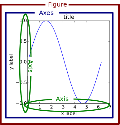
For each plot, there's a tree-like structure of matplotlib objects.

• Figure. The outermost container for a matplotlib graphic, which can contain multiple Axes objects.
• Axes. Actually the individual plot or graph as we think, rather than multiple "axis".
• Below the Axes are smaller objects such as tick marks, individual lines, legends, text boxes.

Stateful vs Stateless Approaches

• Stateful(state-based, state-machine): Directly use plt function, like plt.plot(). Convenient & General.
• Stateless(object-oriented): Use method of Axes object, like ax.plot(). Specific & Customized.

Almost all functions from pyplot such as plt.plot(), are either referring to an existing current Figure and current Axes, or creating new of none exists.

Most of the functions from pyplot also exists as methods of the matplotlib.axes.Axes class. Calling plt.plot() is just more convenient than getting the Axes and calling its plot() method.

Example: plt.title() = plt.gca().set_title(s, *args, **kwargs).

• gca() grabs the current axis and returns it.
• set_title() is a setter method that sets the title for that Axes object.

Subplots

plt.subplots() allows to do more complex plots by using different Axes methods for each ax.

Typical Examples:

• fig, ax = plt.subplots()
• fig, (ax1, ax2) = plt.subplot(nrows=1, ncols=2)

Plot Sub plots with different size:

gridsize = (3, 2)
fig = plt.figure(figsize=(12, 8))
ax1 = plt.subplot2grid(gridsize, (0, 0), colspan=2, rowspan=2)
ax2 = plt.subplot2grid(gridsize, (2, 0))
ax3 = plt.subplot2grid(gridsize, (2, 1))