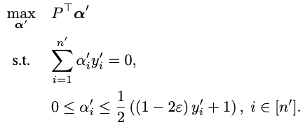
Multi Cost SVM (MC-SVM) is a variant of Support Vector Machines (SVM) designed to accommodate multiple cost scenarios. By introducing multiple weighting parameters
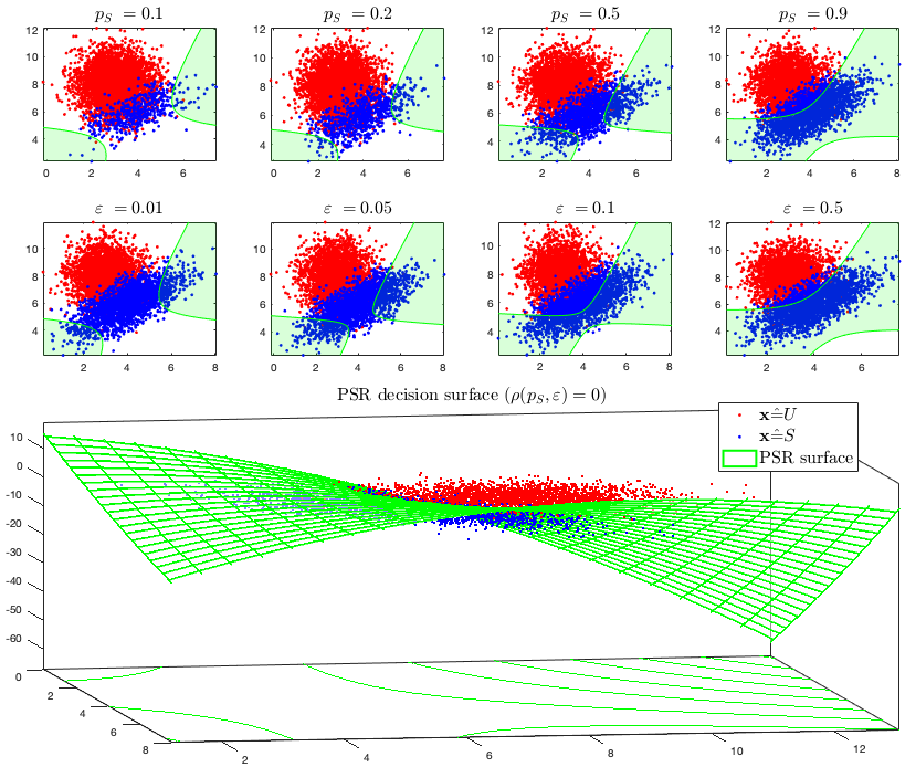
This algorithm was inspired by the concept of Probabilistic Safety Region (PSR)
i.e., the region where in high probability is possible to observe the event
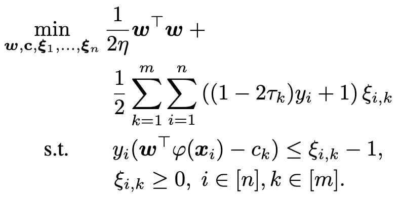
Parameterized Cost Function: MC-SVM incorporates a parameter
System of SVMs: The algorithm constructs a system of
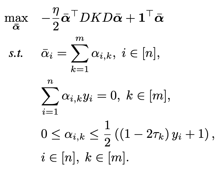
The optimization problem is solved in its dual form
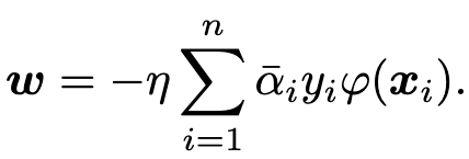
leading to the separation hyperplane
The error in the prediction (false or negative ratio) is then controlled using the following algorithm, based on the quantile regression idea that, discarding the regularization parameter (possible because we computed an independent hyperplane with the algorithm above), the weighting parameter corresponds to the false negative ratio:
To utilize MC-SVM in your projects, follow these steps:
Download the Code: Clone the repository containing the MC-SVM implementation.
Configure Parameters: Adjust the value of
Train the Model: Provide your dataset and train the MC-SVM model using the provided training algorithm.
Evaluate Performance: Evaluate the model's performance on your test dataset and analyze its behavior under different cost scenarios.
Matlab
%%%%%%%%%%%%%%%%%%%%%%%%%%%%%%%%%%%%%%%%%%%%%%%%%%%%%%%%%%%%%%%%%%%%%
For a dataset composed by data sampled with different probabilities
Tau = rand(1,9); m = size(Tau,2);
kernel = 'polynomial';
param = 3;
eta = .001;
alpha_bar = MCSVM_Train(Xtr, Ytr, kernel, param, Tau, eta); # best hyperplane common to all the data
Specializing to a dataset with a known (or estimated) sample probability
%%%%%%%%%%%%%%%%%%%%%%%%%%%%%%%%%%%%%%%%%%%%%%%%%%%%%%%%%%%%%%%%%%%%%
tau = 1-epsilon; # to control the false positives
%%%%%%%%%%%%%%%%%%%%%%%%%%%%%%%%%%%%%%%%%%%%%%%%%%%%%%%%%%%%%%%%%%%%%
alpha_c = SSVM_Train_c(Xtr, Ytr, Xcl_p, Ycl_p, kernel, param, tau, eta, alpha_bar);
b = offset_c(Xtr, Ytr, Xcl_p, Ycl_p, alpha_c, kernel, param, eta, tau, alpha_bar); # best offset that realizes the control of the false positive ration on the desired (calibration) set.
%%%%%%%%%%%%%%%%%%%%%%%%%%%%%%%%%%%%%%%%%%%%%%%%%%%%%%%%%%%%%%%%%%%%%
test
y_pred_ts = SSVM_Test(Xtr, Ytr, Xts_p, alpha_bar, b, 0, kernel, param, eta);
[TPR_SSVM, FPR_SSVM, TNR_SSVM, FNR_SSVM, F1_SSVM, ACC_SSVM] = ConfusionMatrix(Yts_p, y_pred_ts,'on');
disp(['False positive rate:',num2str(FPR_SSVM)])
%%%%%%%%%%%%%%%%%%%%%%%%%%%%%%%%%%%%%%%%%%%%%%%%%%%%%%%%%%%%%%%%%%%%%
Contributions to the MC-SVM algorithm are welcome! Feel free to submit bug reports, feature requests, or pull requests to improve the algorithm's functionality and usability.
