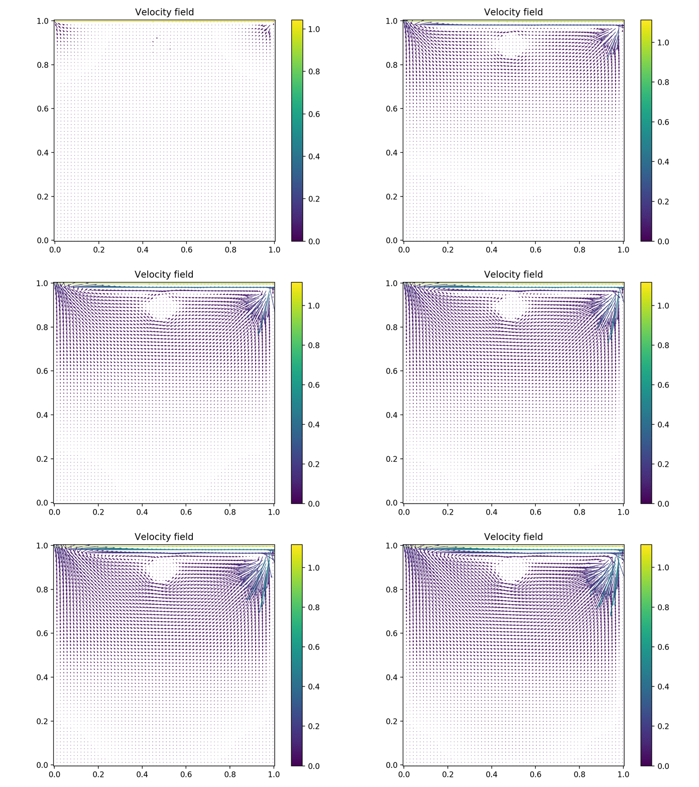
This simulation is implemented in C++ and follows the description given in Numerical simulation in Fluid Dynamics A Practical Introduction by M. Griebel, T. Dornseifer and T. Neunhoeffer.
Example of a top lid moving to the right and driving the flow with it. In addition, there is a circle as an obstacle:

- 2D simulation in a rectangular grid
- Incompressible fluid
- 5 different boundary conditions at the edges of the grid: no-slip, free-slip, outflow, inflow, periodic boundaries
- Obstacles inside the domain
- A python script to visualise the output
- Parallelized computation
- Obstacles moving due to the flow
- 3D simulation
- F and G could be calculated together (so that we have less loops). And then the boundary values for them could be put into one function too.
- Verify the different boundary conditions
All of this was developed on a linux machine and may not work directly on Windows or Mac.
-
mpich package (openMPI, gcc) for compiling and running (even though parallel computation is not implemented yet). I use version 3.3.1-1 of mpich found on the AUR.
-
The libraries numpy, matplotlib and pandas in python to visualise the output. I use python 3.7
A typical run would consist of 3:
- Set the inputs for the desired simulation
- Run the simulation
- Look at the outputs
The input file is located at IO/input:
| Inputs | what it does |
|---|---|
| xlength | length of the system along x |
| ylength | length of the system along y |
| imax | number of cells in x |
| jmax | number of cells in y |
| dt | maximum desired time step |
| t_end | simulation time |
| dt_out | time difference between 2 consecutive simulation dumps |
| tau | security factor (0<tau<=1) for the time step |
| itermax | maximum number of iteration to get the pressure when using the SOR algo. |
| eps | maximum residual in the SOR algo. |
| omega | coeff in the SOR algo |
| Re | Reynolds number |
| gx | external force along x |
| gy | external force along y |
| UI | Initial velocity along x (given in the whole domain) |
| VI | Initial velocity along y (given in the whole domain) |
| PI | Initial pressure (given in the whole domain) |
| rho | density |
| dynvis | dynamical viscosity |
| inflow | speed of the inflow in case of inflow boundary condition |
| wW | boundary condition on the left of the box (x=0) |
| wE | boundary condition on the right of the box (x=xlength) |
| wN | boundary condition on the top of the box (y=ylength) |
| wS | boundary condition on the bottom of the box (y=0) |
The values of rho and dynvis are not currently used. I hesitated between requesting physical inputs values or dimensionless inputs.
Currently the inputs should be dimensionless and the parameters rho and dynvis are hence useless.
The wW, wE, wS, wN can take 5 values: 1, 2, 3 ,4 or 5. A value of:
- 1: indicates the no slip condition i.e. all the velocities vanish at the boundary
- 2: indicates the free slip condition i.e. normal velocity is 0 but the tangential is "free" ($ \frac{\partial \phi_t}{\partial n} = 0 $).
- 3: indicates outflow i.e. the fluid simply gets out of the domain.
- 4: indicates inflow i.e. fluid enters the domain. (There is no current input for the velocity of the flow, it is hard coded in the boundary.cpp file)
- 5: indicates periodic boundaries. For this one to work, the pair wW and wE or the pair wS and wN should be given the value 5.
If you would like more specific boundary conditions, such as a narrow time-dependent inflow, this needs to be implemented in the setSpecBoundaries function in the boundary.cpp file. Doing this will require recompiling the code.
If you would like to include obstacles in the domain, you need to provide a IO/obstacle file that will be read when running the simulation. The data in this file must follow the type of boundary condition as defined in the include/definitions.h file. That is, depending on the obstacle type (no-slip or free-slip) and the orientation of the bins making the obstacle, different values should be given. A template python script can be found in the IO/create_obstacle/create_circle.py . The loop which writes the file is of curcial importance and MUST NOT be changed.
Note: If you change the size of the grid (imax and jmax in IO/input), you must recreate a new obstacle file.
If you edited the code, run:
make
You can now run the code:
make run
Go the the plot directory and run:
./fluid_plot.py
Going into the file (towards the end), you can comment/uncomment the desired plots: time_evolution_imshow or time_evolution_quiver.