Fastor is a smart stack-based high performance tensor (multi-dimensional array) library written in modern C++ [C++11/14/17] with powerful in-built tensor algebraic functionalities (tensor contraction, permutation, reductions, special tensor groups etc). Designed as a generic multi-dimensional tensor algebra library, Fastor also incorporates domain specific features for tensor contraction algorithms typically arising in classical mechanics, in particular, in finite element analysis. There are multiple paradigms that Fastor exploits:
- Operation minimisation/Low FLOP/Complexity reducing Algorithms: Fastor relies on an extremely smart and domain-aware Expression Template (ET) engine that can not only perform lazy evaluations and operator chaining but can also perform sophisticated mathematical transformation or compile time graph optimisation or both to reduce the complexity of evaluation of expressions by orders of magnitude. Some of these functionalities are non-existent in other available C++ ET linear algebra libraries.
- SIMD/Data parallelism/Stream computing Fastor utilises explicit SIMD (SSE/SSE2/SSE3/SSE4/AVX/AVX2/AVX512/FMA) instructions
- Zero overhead tensor algebraic functions statically dispatched bespoke kernels for a variety of tensor products using a priori knowledge of tensors either through template specialisation or advanced topological studies or both
Fastor provides a high level interface for tensor algebra. As a first example consider the following
Tensor<double> scalar; // A scalar
Tensor<double,6> vector6; //  A vector
Tensor<double,4,5> matrix; // A second order tensor
Tensor<double,3,3,3> tensor_3; // A third order tensor with dimension 3x3x3
tensor_3.arange(0); // fill tensor with sequentially ascending numbers
print(tensor_3); // print out the tensor
tensor_3(0,2,1); // index a tensor
tensor_3(all,last,seq(0,2)); // slice a tensor
tensor_3.rank(); // get rank of tensor, 3 in this case
Tensor<float,2,2,2,2,1,2,2,4,3,2,3,3,6> tensor_13; // A 13th order tensor
will output the following
[0,:,:]
⎡      0,       1,       2 ⎤
⎢      3,       4,       5 ⎥
⎣      6,       7,       8 ⎦
[1,:,:]
⎡      9,      10,      11 ⎤
⎢     12,      13,      14 ⎥
⎣     15,      16,      17 ⎦
[2,:,:]
⎡     18,      19,      20 ⎤
⎢     21,      22,      23 ⎥
⎣     24,      25,      26 ⎦
Einstein summation as well as summing over multiple (i.e. more than two) indices are supported. As a complete example, for instance, consider
#include <Fastor.h>
using namespace Fastor;
enum {I,J,K,L,M,N};

int main() {
    // An example of Einstein summation
    Tensor<double,2,3,5> A; Tensor<double,3,5,2,4> B;
    // fill A and B
    A.random(); B.random();
    auto C = einsum<Index<I,J,K>,Index<J,L,M,N>>(A,B);

    // An example of summing over three indices
    Tensor<double,5,5,5> D; D.random();
    auto E = reduction(D);

    // An example of tensor permutation
    Tensor<float,3,4,5,2> F; F.random();
    auto G = permutation<Index<J,K,I,L>>(F);

    // Output the results
    print("Our big tensors:",C,E,G);

    return 0;
}
You can compile and run this by providing the following (or equivalent) flags to your compiler -std=c++14 -O3 -march=native -DNDEBUG.
Fastor introduces powerful tensor views which make tensor indexing, slicing and broadcating look and feel native to scientific programmers. Consider the following examples
Tensor<double,4,3,10> A, B;
A.random(); B.random();
Tensor<double,2,2,5> C; Tensor<double,4,3,1> D;

// Dynamic views -> seq(first,last,step)
C = A(seq(0,2),seq(0,2),seq(0,last,2));                              // C = A[0:2,0:2,0::2]
D = B(all,all,0) + A(all,all,last);                                  // D = B[:,:,0] + A[:,:,-1]
A(2,all,3) = 5.0;                                                    // A[2,:,3] = 5.0

// Static views -> fseq<first,last,step>
C = A(fseq<0,2>(),fseq<0,2>(),fseq<0,last,2>());                     // C = A[0:2,0:2,0::2]
D = B(fall,fall,fseq<0,1>()) + A(fall,fall,fseq<9,10>());            // D = B[:,:,0] + A[:,:,-1]
A(2,fall,3) = 5.0;                                                   // A[2,:,3] = 5.0

// Overlapping is also allowed without having undefined behaviour
A(seq(2,last),all,all).noalias() += A(seq(0,last-2),all,all);        // A[2::,:,:] += A[::-2,:,:]
// Note that in case of perfect overlapping noalias is not required
A(seq(0,last-2),all,all) += A(seq(0,last-2),all,all);                // A[::2,:,:] += A[::2,:,:]

// If instead of a tensor view, one needs an actual tensor the iseq could be used
// iseq<first,last,step>
C = A(iseq<0,2>(),iseq<0,2>(),iseq<0,last,2>());                     // C = A[0:2,0:2,0::2]
// Note that iseq returns an immediate tensor rather than a tensor view and hence cannot appear
// on the left hand side, for instance
A(iseq<0,2>(),iseq<0,2>(),iseq<0,last,2>()) = 2; // Will not compile, as left operand is an rvalue

// One can also index a tensor with another tensor(s)
Tensor<float,10,10> E; E.fill(2);
Tensor<int,5> it = {0,1,3,6,8};
Tensor<size_t,10,10> t_it; t_it.arange();
E(it,0) = 2;
E(it,seq(0,last,3)) /= -1000.;
E(all,it) += E(all,it) * 15.;
E(t_it) -= 42 + E;
Aside from iseq (which pretty much immediately returns another tensor), all other possible combination of slicing and broadcasting types are possible. For instance, one complex slicing and broadcasting example is given below
A(all,all) -= log(B(all,all,0)) + abs(B(all,fall,1)) + sin(C(all,0,all,0)) - 102. - cos(B(all,all,0));It should be mentioned that since tensor views work on a view of (reference to) a tensor and do not copy any data in the background, the use of the keyword auto can be dangerous at times
auto B = A(all,all,seq(0,5),seq(0,3)); // the scope of view expressions ends with ; as view is a refrerence to an rvalue
auto C = B + 2; // Hence this will sigfault as B refers to a non-existing piece of memory
To solve this issue, use immediate construction from a view
Tensor<double,2,2,5,3> B = A(all,all,seq(0,5),seq(0,3)); // B is now permanent
auto C = B + 2; // This will behave as expected
From a performance point of view, Fastor tries very hard to vectorise (read SIMD vectorisation) tensor views, but this heavily depends on the compilers ability to inline multiple recursive functions [as is the case for all expression templates]. If a view appears on the right hand side of an assignment, but not on the left, Fastor automatically vectorises the expression. However if a view appears on the left hand side of an assignment, Fastor does not by default vectorise the expression. To enable vectorisation across all tensor views use the compiler flag -DFASTOR_USE_VECTORISE_EXPR_ASSIGN. Also for performance reasons, it is beneficial to avoid overlapping assignments, otherwise a copy will be made. If your code does not use any overlapping assignments, then this feature can be turned off completely by issusing -DFASTOR_NO_ALIAS. At this stage it is also beneficial to consider that while compiling a complex and big expressions the inlining limit of the compiler should be increased and tested i.e. -finline-limit=<big number> for GCC, -mllvm -inline-threshold=<big number> for Clang and -inline-forceinline for ICC.
As an example to see how efficiently tensor views can be vectorised, consider the following 4th order finite difference example for Laplace equation
Tensor<double,100,100> u, v;
// fill u and v
// A complex assignment expression involving multiple tensor views
u(seq(1,last-1),seq(1,last-1)) =
    ((  v(seq(0,last-2),seq(1,last-1)) + v(seq(2,last),seq(1,last-1)) +
        v(seq(1,last-1),seq(0,last-2)) + v(seq(1,last-1),seq(2,last)) )*4.0 +
        v(seq(0,last-2),seq(0,last-2)) + v(seq(0,last-2),seq(2,last)) +
        v(seq(2,last),seq(0,last-2))   + v(seq(2,last),seq(2,last)) ) / 20.0;
using GCC 6.2 with -O3 -mavx2 -mfma -finline-limit=100000 -ffp-contract=fast -DNDEBUG -DFASTOR_NO_ALIAS -DFASTOR_USE_VECTORISE_EXPR_ASSIGN the above expression compiles to
L129:
  leaq  -768(%rcx), %rdx
  movq  %rsi, %rax
  .align 4,0x90
L128:
  vmovupd 8(%rax), %ymm0
  vmovupd (%rax), %ymm1
  addq  $32, %rdx
  addq  $32, %rax
  vaddpd  1576(%rax), %ymm0, %ymm0
  vaddpd  768(%rax), %ymm0, %ymm0
  vaddpd  784(%rax), %ymm0, %ymm0
  vfmadd132pd %ymm3, %ymm1, %ymm0
  vaddpd  -16(%rax), %ymm0, %ymm0
  vaddpd  1568(%rax), %ymm0, %ymm0
  vaddpd  1584(%rax), %ymm0, %ymm0
  vdivpd  %ymm2, %ymm0, %ymm0
  vmovupd %ymm0, -32(%rdx)
  cmpq  %rdx, %rcx
  jne L128
  vmovupd 2376(%rsi), %xmm0
  vaddpd  776(%rsi), %xmm0, %xmm0
  addq  $800, %rcx
  addq  $800, %rsi
  vaddpd  768(%rsi), %xmm0, %xmm0
  vaddpd  784(%rsi), %xmm0, %xmm0
  vfmadd213pd -32(%rsi), %xmm5, %xmm0
  vaddpd  -16(%rsi), %xmm0, %xmm0
  vaddpd  1568(%rsi), %xmm0, %xmm0
  vaddpd  1584(%rsi), %xmm0, %xmm0
  vdivpd  %xmm4, %xmm0, %xmm0
  vmovups %xmm0, -800(%rcx)
  cmpq  %r13, %rcx
  jne L129
As can be observed, the compiler emits unaligned load and store instructions, but the rest of the generated code is extremely efficient (it does not get more efficient than this). For stack allocated and small tensors the unaligned load/store operations should not be a bottleneck either, as the data would potentially fit in L1 cache. With the help of an optimising compiler, Fastor's functionalities come closest to the ideal metal performance for numerical tensor algebra code.
Fastor is essentially designed for small mutlidimensional tensors (for instance, tensors appearing during numerical integration in a finite element framework such as stresses, work conjugates, Hessian or small multi-dimensional arrays useful for 2D/3D graphics). As can be seen from the above examples, Fastor is based on fixed size static arrays (entirely stack allocation). The dimensions of the tensors must be known at compile time, which is typically the case for the use-cases it is designed for. However one of the strongest features of Fastor is in its in-built template meta-programming engine, in that, it can automatically determine at compile time, the dimensions of the tensors resulting from a complex operation yet to be performed, hence it can always allocate exactly the right amount of stack memory required. This is in contrast to static arrays in C or Fortran where one has to allocate a huge block of memory before hand to avoid stack overflow.
This is a strong statement to make, but Fastor strives to generate optimised SIMD code by utilising the static nature of tensors and the SFINAE (Substitution Failure Is Not an Error) feature of C++11 to statically dispatch calls to bespoke kernels, which completely avoids the need for runtime branching. For example the double contraction of two second order double precision tensors A and B, A_ij*B_ij with dimensions 2x2, is statically dispatched to
return _mm256_sum_pd(_mm256_mul_pd(_mm256_load_pd(A._data),_mm256_load_pd(B._data)));(Notice that the double contraction of two second order tensors of 2x2 requires 4 multiplication + 3 addition which using SIMD lanes can be reduced to 1 multiplication + 1 addition. Also _mm256_sum_pd is Fastor's in-built extension to SIMD intrinsics.) while for 3x3 double precision second order tensors the call is dispatched to
__m256d r1 = _mm256_mul_pd(_mm256_load_pd(A._data),_mm256_load_pd(B._data));
__m256d r2 = _mm256_mul_pd(_mm256_load_pd(A._data+4),_mm256_load_pd(B._data+4));
__m128d r3 = _mm_mul_sd(_mm_load_sd(A._data+8),_mm_load_sd(B._data+8));
__m128d summ = _mm_add_pd(_add_pd(r3),_add_pd(_mm256_add_pd(r1,r2)));
return _mm_cvtsd_f64(summ);
without the need for a branch or a potential jmp instruction in assembly (again note that 9 multiplication + 8 addition is reduced to 3 multiplication + 3 addition). The main motivation behind customising/optimising these operations for such small tensors is that they are typically needed in the critical hotspots of computer graphics and finite element algorithm, for instance.
A must have feature of every numerical linear algebra and even more so tensor contraction frameworks is lazy evaluation of arbitrary chained operations. Consider the following expression
Tensor<float,16,16,16,16> tn1 ,tn2, tn3, tn4;
tn1.random(); tn2.random(); tn3.random();
tn4 = 2*tn1+sqrt(tn2-tn3);
The above code is transparently converted to a single AVX loop
for (size_t i=0; i<tn4.Size; i+=tn4.Stride)
    _mm256_store_ps(tn4._data+i,_mm256_set1_ps(static_cast<float>(2))*_mm256_load_ps(tn1._data+i)+
    _mm256_sqrt_ps(_mm256_sub_ps(_mm256_load_ps(tn2._data+i),_mm256_load_ps(tn3._data+i)));
avoiding any need for temporary memory allocation. As a DSL, Fastor has a much deeper understanding of the domain. By employing template metaprogrommaing techniques it ventures into the realm of smart expression templates to mathematically transform expression and/or apply compile time graph optimisation to find optimal contraction indices of complex tensor networks. As an example, the trace(matmul(transpose(A),B)) which is O(n^3) in computational complexity is determined to be inefficient and Fastor statically dispatches the call to an equivalent but much more efficient routine, in this case A_ijB_ij or doublecontract(A,B) which is O(n^2). Further examples of such mathemtical transformation include (not inclusive)
// the l in-front of the names stands for 'lazy'
ldeterminant(linverse(A)); // transformed to 1/ldeterminant(A), O(n^3) reduction in computation
ltranspose(lcofactor(A));  // transformed to ladjoint(A), O(n^2) reduction in memory access
ltranspose(ladjoint(A));   // transformed to lcofactor(A), O(n^2) reduction in memory access
lmatmul(lmatmul(A,B),b);   // transformed to lmatmul(A,lmatmul(B,b)), O(n) reduction in computation
// and many more
Note that there are situations that the user may write a complex chain of operations in the most verbose way, perhaps for readibility purposes, but Fastor delays the evaluation of the expression and checks if an equivalent but efficient expression can be computed. The computed expression always binds back to the base tensor, overhead free without a runtime (virtual table/pointer) penalty.
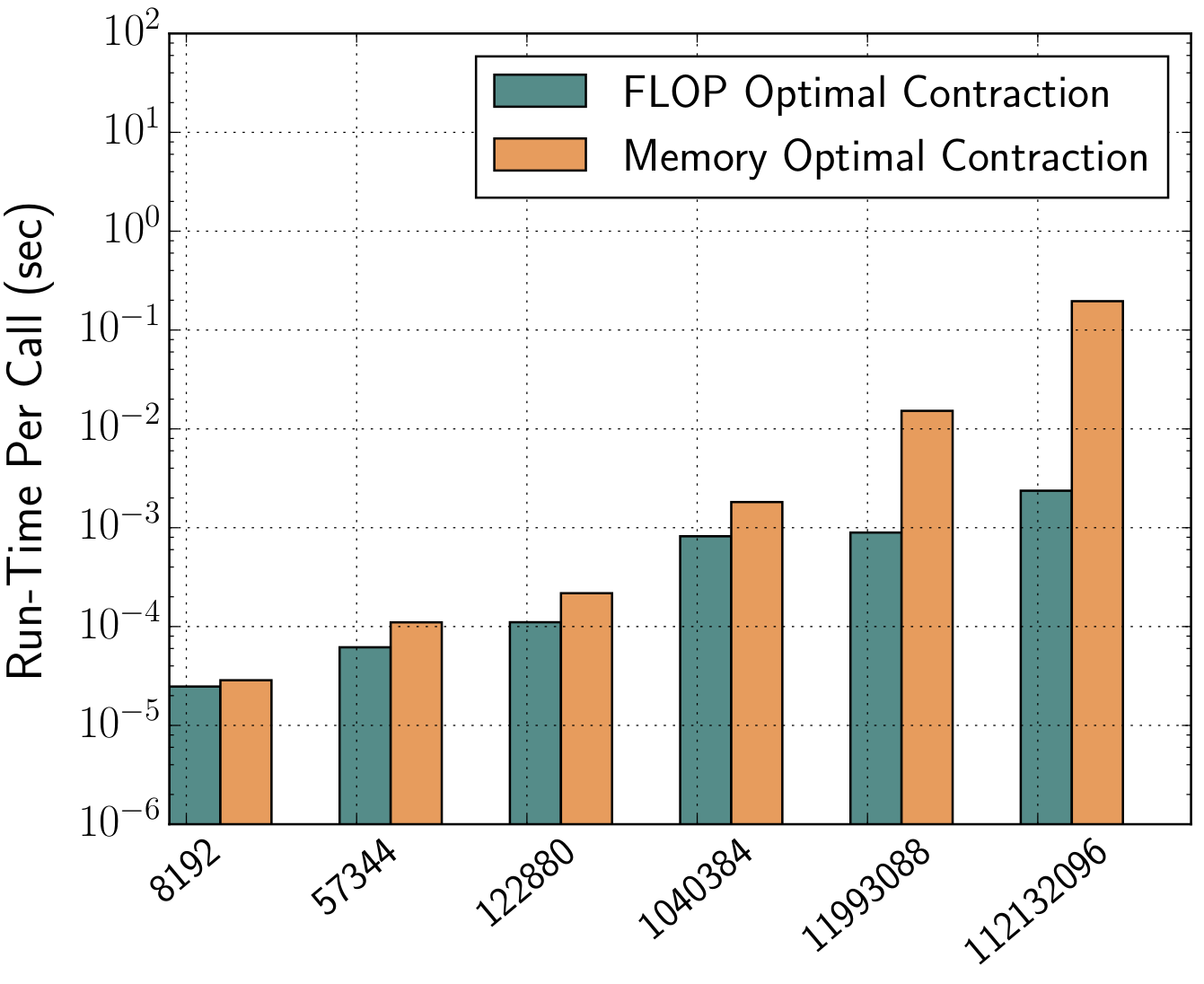
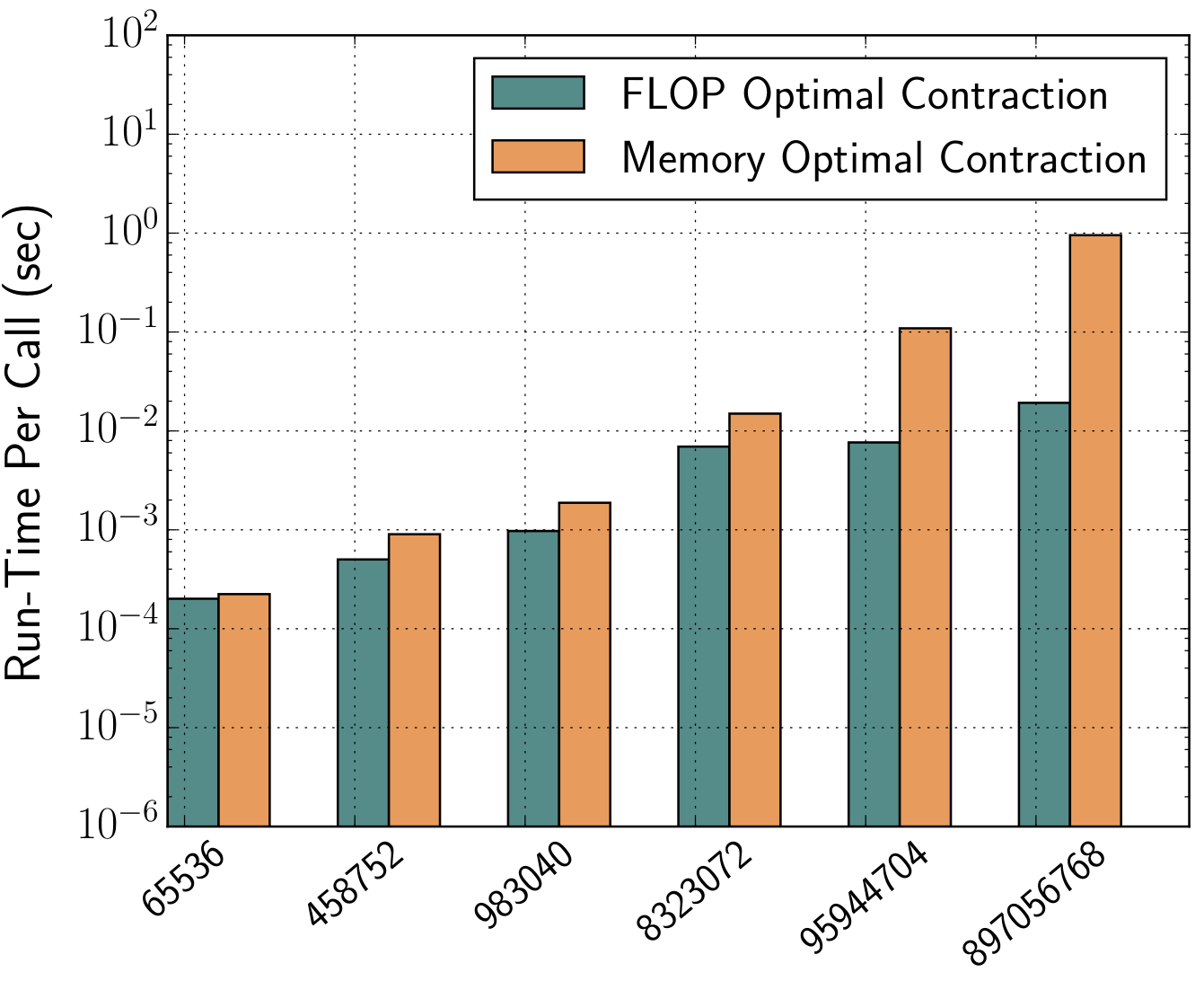
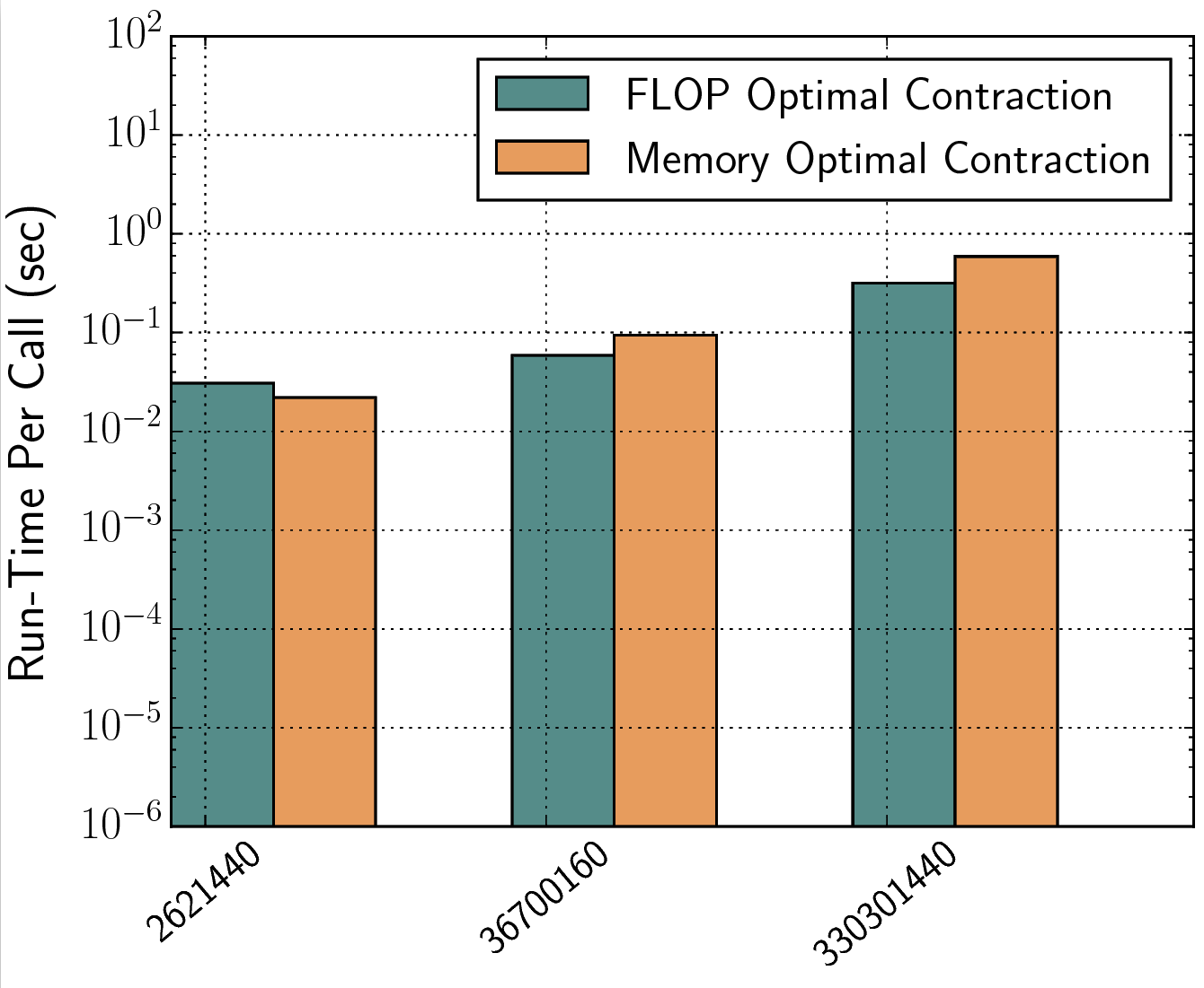
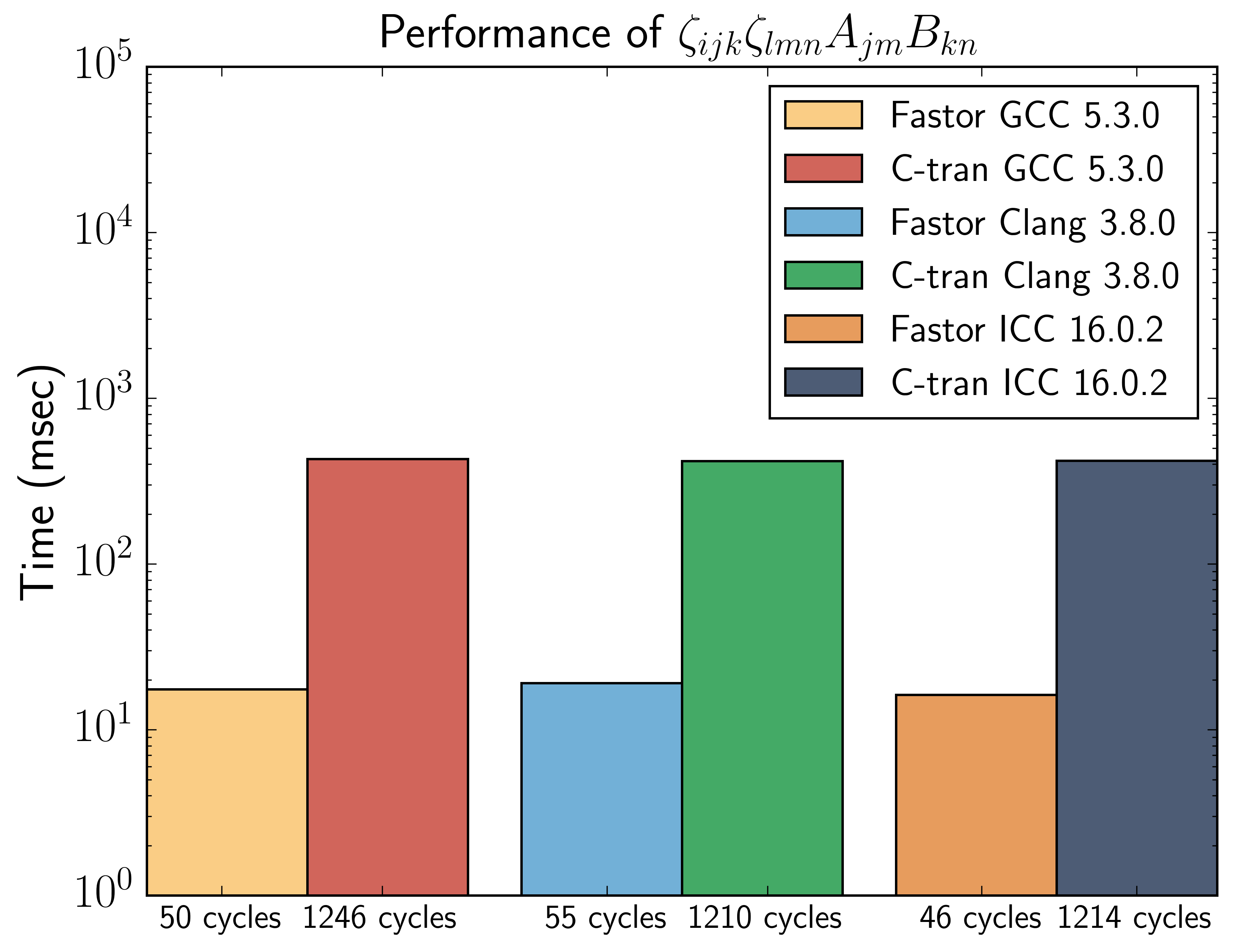
For tensor networks comprising of many higher rank tensors, a full generalisation of the above mathematical transformation can be performed through a constructive graph search optimisation. This typically involves finding the most optimal pattern of tensor contraction by studying the indices of contraction wherein tensor pairs are multiplied, summed over and factorised out in all possible combinations in order to come up with a cost model. Once again, knowing the dimensions of the tensor and the contraction pattern, Fastor performs this operation minimisation step at compile time and further checks the SIMD vectorisability of the tensor contraction loop nest (i.e. full/partial/broadcast vectorisation). In nutshell, it not only minimises the the number of floating point operations but also generates the most optimum vectorisable loop nest for computing those FLOPs. The following figures show the run time benefit of operation minimisation (FLOP optimal) over a single expression evaluation (Memory-saving) approach in contracting a three-tensor-network fitting in L1, L2 and L3 caches, respectively
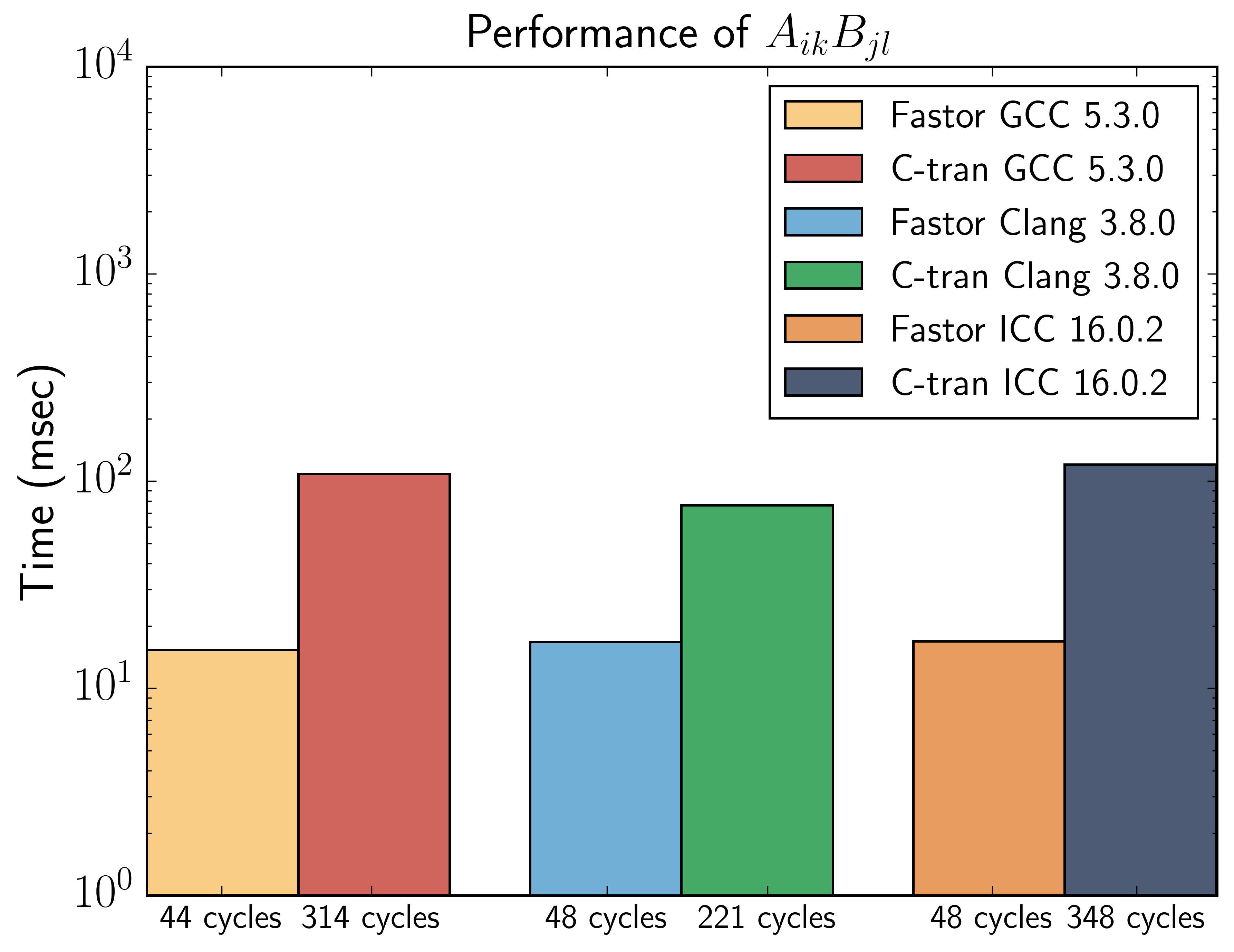
In nonlinear mechanics, it is customary to transform high order tensors to low rank tensors using Voigt transformation. Fastor has domain-specific features for such tensorial operations. For example, consider the dyadic product A_ik*B_jl, that can be computed in Fastor like
Tensor<double,3,3> A,B;
A.random(); B.random();
Tensor<double,6,6> C = einsum<Index<0,2>,Index<1,3>,FASTOR_Voigt>(A,B);
// or alternatively
enum {I,J,K,L};
Tensor<double,6,6> D = einsum<Index<I,K>,Index<J,L>,FASTOR_Voigt>(A,B);
As you notice, all indices are resolved and the Voigt transformation is performed at compile time, keeping only the cost of computation at runtime. Equivalent implementation of this in C/Fortran requires either low-level for loop style programming that has an O(n^4) computational complexity and non-contiguous memory access, or if a function like einsum is desired the indices will need to be passed requiring potentially extra register allocation. Here is performance benchmark between Ctran (C/Fortran) for loop code and the equivalent Fastor implementation for the above example, run over a million times (both compiled using -O3 -mavx, on Intel(R) Xeon(R) CPU E5-2650 v2 @2.60GHz running Ubuntu 14.04):
Notice that by compiling with the same flags, it is meant that the compiler is permitted to auto-vectorise the C/tran code as well. The real performance of Fastor comes from the fact, that when a Voigt transformation is requested, Fastor does not compute the elements which are not needed.
Building upon its domain specific features, Fastor implements the tensor cross product family of algebra recently introduced by Bonet et. al. in the context of numerical analysis of nonlinear classical mechanics which can significantly reduce the amount algebra involved in tensor derivatives of functionals which are forbiddingly complex to derive using a standard approach. The tensor cross product of two second order tensors is defined as C_iI = e_ijk*e_IJK*A_jJ*b_kK where e is the third order permutation tensor. As can be seen this product is O(n^6) in computational complexity (furthermore a cross product is essentially defined in 3-dimensional space i.e. perfectly suitable for stack allocation). Using Fastor the equivalent code is only 81 SSE intrinsics
// A and B are second order tensors
using Fastor::LeviCivita_pd;
Tensor<double,3,3> E = einsum<Index<i,j,k>,Index<I,J,K>,Index<j,J>,Index<k,K>>
                       (LeviCivita_pd,LeviCivita_pd,A,B);
// or simply
Tensor<double,3,3> F = cross(A,B);
Here is performance benchmark between Ctran (C/Fortran) code and the equivalent Fastor implementation for the above example, run over a million times (both compiled using -O3 -mavx, on Intel(R) Xeon(R) CPU E5-2650 v2 @2.60GHz running Ubuntu 14.04):
Notice the almost two orders of magnitude performance gain using Fastor. Again the real performance gain comes from the fact that Fastor eliminates zeros from the computation.
A set of boolean tensor routines are available in Fastor. Note that, whenever possible most of these operations are performed at compile time
is_uniform();   // does the tensor span equally in all spatial dimensions, generalisation of square matrices
is_orthogonal();
does_belong_to_sl3(); // does the tensor belong to special linear 3D group
does_belong_to_so3(); // does the tensor belong to special orthogonal 3D group
is_symmetric(int axis_1, int axis_2); // is the tensor symmetric in the axis_1 x axis_2 plane
is_equal(B); // equality check with another tensor
is_identity();All basic numerical linear algebra subroutines for small tensors (where the overhead of calling vendor/optimised BLAS is typically not worth it) are fully SIMD optimised and efficiently implemented
Tensor<double,3,3> A,B;
// fill A and B
auto ab = matmul(A,B);          // matrix matrix multiplication of A*B
auto a_norm = norm(A);          // Frobenious norm of A
auto b_det = determinant(B);    // determinant of B
auto a_inv = inverse(A);        // inverse of A
auto b_cof = cofactor(B); // cofactor of BFastor utilises a bunch of meta-functions to perform most operations at compile time, consider the following examples
Tensor<double,3,4,5> A;
Tensor<double,5,3,4> B;
Tensor<double,3,3,3> C;
auto D = permutation<Index<2,0,1>>(A); // type of D is deduced at compile time as Tensor<double,5,3,4>
auto E = einsum<Index<I,J,K>,Index<L,M,N>>(D,B); // type of E is deduced at compile time as Tensor<double,5,3,4,5,3,4>
auto F = einsum<Index<I,I,J>>(C); // type of F is deduced at compile time as Tensor<double,3>
auto F2 = reduction(C); // type of F2 is deduced at compile time as scalar i.e. Tensor<double>
auto E2 = reduction(D,B); // type of E2 is deduced at compile time as Tensor<double>
Tensor<float,2,2> G,H;
trace(H); // trace of H, in other words H_II
reduction(G,H); // double contraction of G and H i.e. G_IJ*H_IJ
As you can observe with combination of permutation, contraction, reduction and einsum (which itself is a glorified wrapper over the first three) any type of tensor contraction, and permutation is possible, and using meta-programming the right amount of stack memory to be allocated is deduced at compile time.
Fastor is extremely light weight, it is a header-only library, requires no build or compilation process and has no external dependencies. It is written in pure C++11 from the foundation.
Fastor has been tested against the following compilers (on Ubuntu 14.04/16.04/18.04 and macOS). While compiling on macOS with Clang, -std=c++14 is necessary
- GCC 4.8, GCC 4.9, GCC 5.1, GCC 5.2, GCC 5.3, GCC 5.4, GCC 6.2, GCC 7.3, GCC 9.1
- Clang 3.6, Clang 3.7, Clang 3.8, Clang 3.9, Clang 5
- Intel 16.0.1, Intel 16.0.2, Intel 16.0.3, Intel 17.0.1, Intel 18.2
Fastor can be cited as
@Article{Poya2017,
    author="Poya, Roman and Gil, Antonio J. and Ortigosa, Rogelio",
    title = "A high performance data parallel tensor contraction framework: Application to coupled electro-mechanics",
    journal = "Computer Physics Communications",
    year="2017",
    doi = "http://dx.doi.org/10.1016/j.cpc.2017.02.016",
    url = "http://www.sciencedirect.com/science/article/pii/S0010465517300681"
}
Similar projects exist with varying levels of functionality, in particular
- FTensor: Dense tensor algebra framework for up to rank 4 tensors
- LTensor: Dense tensor algebra framework for up to rank 4 tensors
- libtensor: Dense tensor algebra framework for up to rank 6 tensors
- Eigen's tensor algebra package: Arbitrary rank dense tensor algebra module
- Blitz++'s tensor module: Dense linear algebra framework for up to rank 11 tensors
- TiledArray: Massively parallel arbitrary rank block sparse tensor algebra framework based on Eigen
- Cyclops Tensor Framework: Distributed memory arbitrary rank sparse tensor algebra framework
