Flower Classification

About the dataset

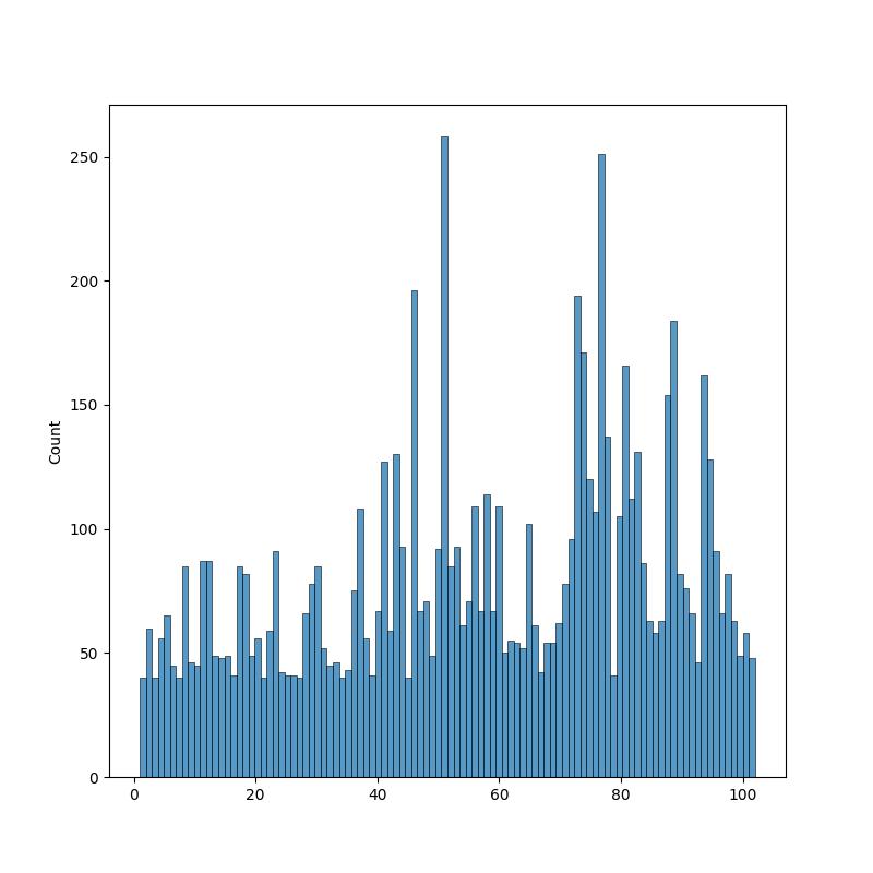
We have created a 102 category dataset, consisting of 102 flower categories. The flowers chosen to be commonly occuring in the United Kingdom. Each class consists of between 40 and 258 images. We have a dataset of 102 classes of flowers that are commonly found in the United Kingdom. Each class consists of between 40 and 258 images (total number of samples is 8189). Table1 shows, number of sample for each class.

Label	Name	Count	Label	Name	Count
0	pink primrose	85	51	wild pansy	85
1	hard-leaved pocket orchid	93	52	primula	93
2	canterbury bells	61	53	sunflower	61
3	sweet pea	71	54	pelargonium	71
4	english marigold	109	55	bishop of llandaff	109
5	tiger lily	67	56	gaura	67
6	moon orchid	114	57	geranium	114
7	bird of paradise	67	58	orange dahlia	67
8	monkshood	109	59	pink-yellow dahlia?	109
9	globe thistle	50	60	cautleya spicata	50
10	snapdragon	55	61	japanese anemone	55
11	colt's foot	54	62	black-eyed susan	54
12	king protea	52	63	silverbush	52
13	spear thistle	102	64	californian poppy	102
14	yellow iris	61	65	osteospermum	61
15	globe-flower	42	66	spring crocus	42
16	purple coneflower	54	67	bearded iris	54
17	peruvian lily	54	68	windflower	54
18	balloon flower	62	69	tree poppy	62
19	giant white arum lily	78	70	gazania	78
20	fire lily	96	71	azalea	96
21	pincushion flower	194	72	water lily	194
22	fritillary	171	73	rose	171
23	red ginger	120	74	thorn apple	120
24	grape hyacinth	107	75	morning glory	107
25	corn poppy	251	76	passion flower	251
26	prince of wales feathers	137	77	lotus	137
27	stemless gentian	41	78	toad lily	41
28	artichoke	105	79	anthurium	105
29	sweet william	166	80	frangipani	166
30	carnation	112	81	clematis	112
31	garden phlox	131	82	hibiscus	131
32	love in the mist	86	83	columbine	86
33	mexican aster	63	84	desert-rose	63
34	alpine sea holly	58	85	tree mallow	58
35	ruby-lipped cattleya	63	86	magnolia	63
36	cape flower	154	87	cyclamen	154
37	great masterwort	184	88	watercress	184
38	siam tulip	82	89	canna lily	82
39	lenten rose	76	90	hippeastrum	76
40	barbeton daisy	66	91	bee balm	66
41	daffodil	46	92	ball moss	46
42	sword lily	162	93	foxglove	162
43	poinsettia	128	94	bougainvillea	128
44	bolero deep blue	91	95	camellia	91
45	wallflower	66	96	mallow	66
46	marigold	82	97	mexican petunia	82
47	buttercup	63	98	bromelia	63
48	oxeye daisy	49	99	blanket flower	49
49	common dandelion	58	100	trumpet creeper	58
50	petunia	48	101	blackberry lily	48

Table1: This table shows the number of samples for each class

According to the distribution at figure1, it is clear that classes have imbalanced samples which has been a challenge to work with this dataset.

Figure1: This plot shows the distribution of samples for each class

Figure2: Shows one sample from each category from the dataset

Dataset can be downloaded from this website

Final result

Label	Name	Precision	Recall	F1-score	support
0	pink primrose	1.00	1.00	1.00	8
1	hard-leaved pocket orchid	1.00	1.00	1.00	12
2	canterbury bells	1.00	0.88	0.93	8
3	sweet pea	1.00	1.00	1.00	11
4	english marigold	1.00	1.00	1.00	13
5	tiger lily	1.00	1.00	1.00	9
6	moon orchid	0.89	1.00	0.94	8
7	bird of paradise	1.00	1.00	1.00	17
8	monkshood	0.90	1.00	0.95	9
9	globe thistle	1.00	1.00	1.00	9
10	snapdragon	1.00	1.00	1.00	17
11	colt's foot	1.00	1.00	1.00	17
12	king protea	1.00	1.00	1.00	9
13	spear thistle	1.00	1.00	1.00	9
14	yellow iris	1.00	1.00	1.00	9
15	globe-flower	1.00	1.00	1.00	8
16	purple coneflower	1.00	1.00	1.00	17
17	peruvian lily	1.00	1.00	1.00	16
18	balloon flower	1.00	1.00	1.00	9
19	giant white arum lily	1.00	1.00	1.00	11
20	fire lily	1.00	1.00	1.00	8
21	pincushion flower	1.00	1.00	1.00	11
22	fritillary	1.00	1.00	1.00	18
23	red ginger	1.00	1.00	1.00	8
24	grape hyacinth	0.88	0.88	0.88	8
25	corn poppy	1.00	1.00	1.00	8
26	prince of wales feathers	1.00	1.00	1.00	8
27	stemless gentian	1.00	1.00	1.00	13
28	artichoke	1.00	1.00	1.00	15
29	sweet william	1.00	1.00	1.00	17
30	carnation	0.91	1.00	0.95	10
31	garden phlox	1.00	1.00	1.00	9
32	love in the mist	1.00	1.00	1.00	9
33	mexican aster	1.00	1.00	1.00	8
34	alpine sea holly	1.00	1.00	1.00	8
35	ruby-lipped cattleya	1.00	1.00	1.00	15
36	cape flower	1.00	1.00	1.00	21
37	great masterwort	1.00	1.00	1.00	11
38	siam tulip	1.00	1.00	1.00	8
39	lenten rose	1.00	0.85	0.92	13
40	barbeton daisy	1.00	1.00	1.00	25
41	daffodil	1.00	1.00	1.00	11
42	sword lily	0.96	1.00	0.98	26
43	poinsettia	1.00	1.00	1.00	18
44	bolero deep blue	1.00	1.00	1.00	8
45	wallflower	0.97	1.00	0.99	39
46	marigold	1.00	1.00	1.00	13
47	buttercup	1.00	1.00	1.00	14
48	oxeye daisy	1.00	1.00	1.00	9
49	common dandelion	1.00	1.00	1.00	18
50	petunia	1.00	1.00	1.00	51
51	wild pansy	1.00	1.00	1.00	17
52	primula	0.95	1.00	0.97	18
53	sunflower	1.00	1.00	1.00	12
54	pelargonium	1.00	1.00	1.00	14
55	bishop of llandaff	1.00	1.00	1.00	21
56	gaura	0.93	1.00	0.96	13
57	geranium	1.00	0.95	0.98	22
58	orange dahlia	1.00	1.00	1.00	13
59	pink-yellow dahlia?	1.00	1.00	1.00	21
60	cautleya spicata	1.00	1.00	1.00	10
61	japanese anemone	1.00	1.00	1.00	11
62	black-eyed susan	1.00	1.00	1.00	10
63	silverbush	1.00	1.00	1.00	10
64	californian poppy	1.00	1.00	1.00	20
65	osteospermum	1.00	1.00	1.00	12
66	spring crocus	1.00	1.00	1.00	8
67	bearded iris	1.00	1.00	1.00	10
68	windflower	1.00	1.00	1.00	10
69	tree poppy	1.00	1.00	1.00	12
70	gazania	1.00	1.00	1.00	15
71	azalea	0.95	1.00	0.97	19
72	water lily	1.00	1.00	1.00	38
73	rose	1.00	0.97	0.99	34
74	thorn apple	1.00	1.00	1.00	24
75	morning glory	1.00	1.00	1.00	21
76	passion flower	1.00	1.00	1.00	50
77	lotus	1.00	1.00	1.00	27
78	toad lily	1.00	1.00	1.00	8
79	anthurium	1.00	1.00	1.00	21
80	frangipani	1.00	1.00	1.00	33
81	clematis	1.00	1.00	1.00	22
82	hibiscus	1.00	0.96	0.98	26
83	columbine	0.94	1.00	0.97	17
84	desert-rose	1.00	1.00	1.00	12
85	tree mallow	1.00	1.00	1.00	11
86	magnolia	0.92	1.00	0.96	12
87	cyclamen	0.97	1.00	0.98	30
88	watercress	1.00	1.00	1.00	36
89	canna lily	1.00	1.00	1.00	16
90	hippeastrum	1.00	1.00	1.00	15
91	bee balm	1.00	0.92	0.96	13
92	ball moss	0.90	1.00	0.95	9
93	foxglove	1.00	0.91	0.95	32
94	bougainvillea	1.00	0.92	0.96	25
95	camellia	0.94	0.89	0.91	18
96	mallow	0.87	1.00	0.93	13
97	mexican petunia	1.00	0.94	0.97	16
98	bromelia	1.00	1.00	1.00	12
99	blanket flower	1.00	1.00	1.00	9
100	trumpet creeper	1.00	1.00	1.00	11
101	blackberry lily	1.00	1.00	1.00	9
Table2: Final results from classification report

Preprocessing

Images are resized to have the shape of (224, 224, 3); this image size is almost compatible with all pretrained models and retains the quality. (Also resize method is bicubic)

The fact that we have a small dataset with imbalanced data, we should definitely consider augmentation. Augmentation parameters are listed below in order:

Random JPEG quality with interval of $[50, 100]$
Random contrast with lower and upper factor of 0.6 and 1.2 respectively
Random horizontal flip
Random brightness with max_delta = 0.3
Random saturation with lower and upper factor of 0.6 and 1.2 respectively
Note that the image should be clipped so to have values from 0 to 255

It has been seen that augmenting prior to resizing results in a better performance but slows the process of training (in our case, it slowed down the process x4 times using Nvidia RTX 2060 notebook)

Since EfficientNetV2B0 is used as the base network, we also used its associate preprocessing input function; training and validation have:

Training
- MAX: 255.0
- MIN: 0.0
- MEAN: 91.89
- STD: 64.52
Validation
- MAX: 255.0
- MIN: 0.0
- MEAN: 93.06
- STD: 70.38

Although the model it self has a preprocessing layer (Rescaling layer) that makes the input in the range of $[-1, 1]$

Model

Given the small dataset, model is trained better with transfer learning. Trying different models, EfficientNetV2B0 has been the best model in both terms of running time and memory and accuracy. Table2 shows layers and parameters for our model.

Layer (Type)	Output Shape	Param #
input_2 (InputLayer)	[(None, 224, 224, 3)]	0
efficientnetv2-b0 (Functional)	(None, 7, 7, 1280)	5919312
global_average_pooling2d (GlobalAveragePooling2D)	(None, 1280)	0
dropout (Dropout)	(None, 1280)	0
dense (Dense)	(None, 102)	130662

Total params: 6,049,974 (23.08 MB)
Trainable params: 5,564,410 (21.23 MB)
Non-trainable params: 485564 (1.85 MB)

Given the fact that number of parameters for training is about $\approx 5M$, it is impossible to gain a good performance without having to deal with the problem of high variance (over fitting) unless we use a large dropout rate (in our case we chose 0.7).

Address the problem of imbalanced data

To address the problem of imbalanced data, we specified weights for each class (to be applied to the loss function). Weights are calculated with:

$$ \begin{equation} w_{i} = \frac{\sum_{j}c_j}{102 c_i } \end{equation} $$

Where $w_i$ denotes the weight for class $i$ and $c_i$ denotes the number of samples for class $i$.

Model compile

One way to address the problem of imbalanced classses, is to use Focal loss. Focal loss applies a modulating term to the cross entropy loss in order to focus learning on hard misclassified examples. It is a dynamically scaled cross entropy loss, where the scaling factor decays to zero as confidence in the correct class increases. Focal loss reduces the contribution of easy examples to the loss function, thereby giving more importance to difficult examples. Helps in dealing with noisy data: In real-world scenarios, the training data may be noisy, which can lead to misclassification.

Note that $\alpha$ should be a list of weights for each class to address the issue of imbalanced classes.

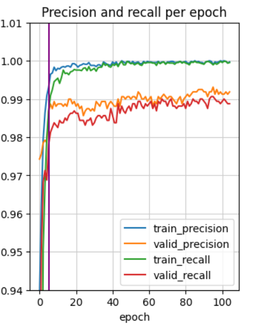
However we did not train via Focal Loss and just weighted the Categorical Crossentropy loss. But both choices resulted in accuracy $\ge 0.98$. But we found latter more promising.

Results

After fine-tuning (freezing up to 149 layers), we've got

	precision	recall	f1-score	support
accuracy			0.99	1602
macro avg	0.99	0.99	0.99	1602
weighted avg	0.99	0.99	0.99	1602

Table3: Classification report

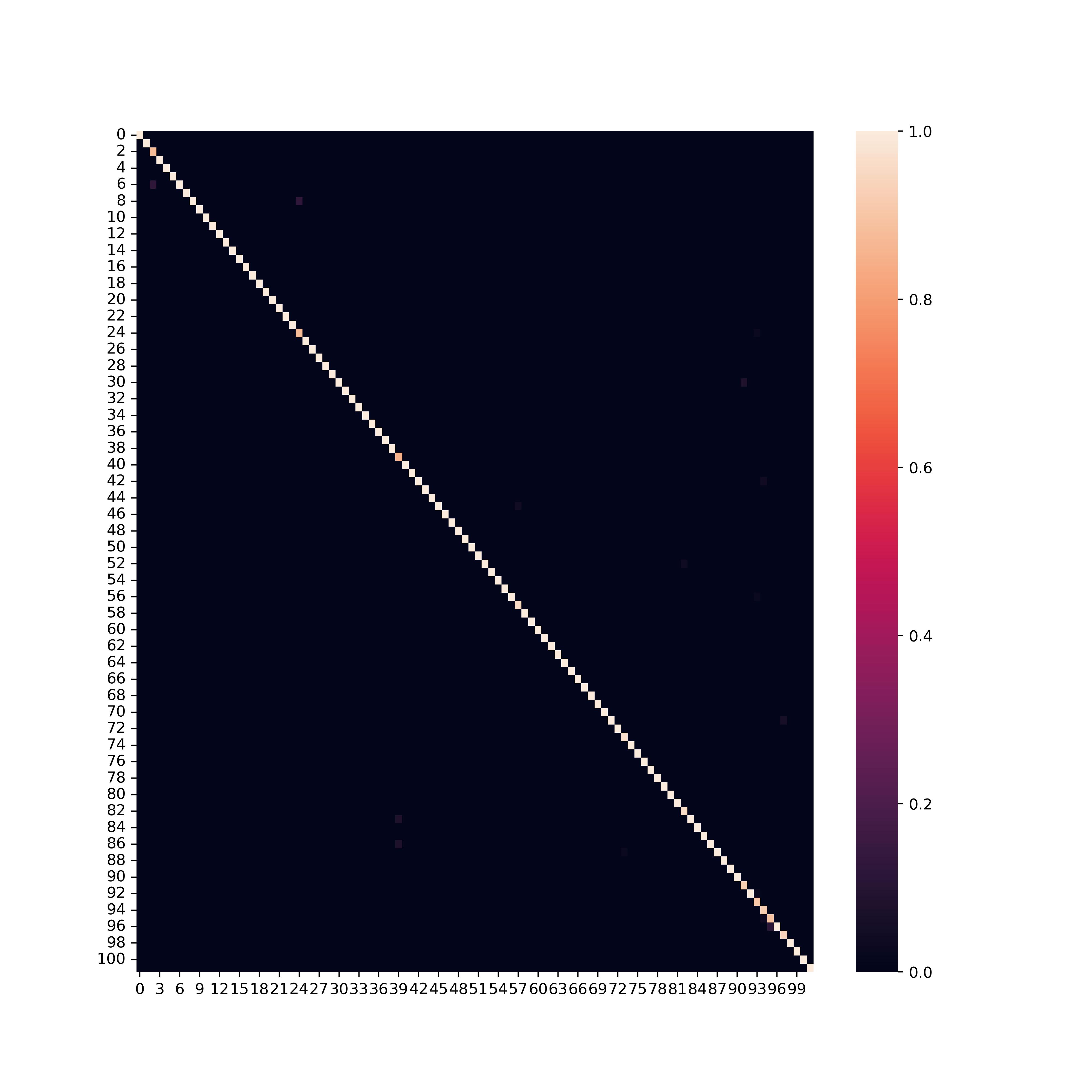
And this is the confusion matrix:

Also result are illlustrated in table2

Model can be downloaded from here

Android implementation

The model is implemented in a simple android program (source code) (release v1.2)

AlirezaKamyab/Flower_Classification