University of Pennsylvania, CIS 565: GPU Programming and Architecture, Project 3
- Aman Sachan
- Tested on: Windows 10, i7-7700HQ @ 2.8GHz 32GB, GTX 1070(laptop GPU) 8074MB (Personal Machine: Customized MSI GT62VR 7RE)
In this project, I implemented a simple CUDA Monte Carlo path tracer. Although path tracers are typically implemented on the CPU, path tracing itself is a highly parallel algorithm if you think about it. For every pixel on the image, we cast a ray into the scene and track its movements until it reaches a light source, yielding a color on our screen. Each ray is dispatched as its own thread, for which intersections and material contributions are processed on the GPU.
More Feature filled Path Tracer I made but on the CPU can be found here.
Monte Carlo Path tracing is a rendering technique that aims to represent global illumination as accurately as possible with respect to reality. The algorithm does this by approximating the integral over all the illuminance arriving at a point in the scene. A portion of this illuminance will go towards the viewpoint camera, and this portion of illuminance is determined by a surface reflectance function (BRDF). This integration procedure is repeated for every pixel in the output image. When combined with physically accurate models of surfaces, accurate models light sources, and optically-correct cameras, path tracing can produce still images that are indistinguishable from photographs.
Path tracing naturally simulates many effects that have to be added as special cases for other methods (such as ray tracing or scanline rendering); these effects include soft shadows, depth of field, motion blur, caustics, ambient occlusion, and indirect lighting, etc.
Due to its accuracy and unbiased nature, path tracing is used to generate reference images when testing the quality of other rendering algorithms. In order to get high quality images from path tracing, a large number of rays must be traced to avoid visible noisy artifacts.


Subsurface BxDF and Specular BRDF on a violet sphere

Lambertian Reference for the image below

Subtle Subsurface Scattering with a scattering coefficient of 300; Entire coloration is due to the subsurface BxDF

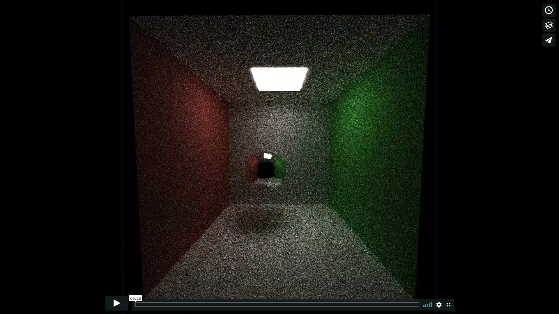
Object infront of the only light source in the scene. Another example of Subsurface Scattering with a scattering coefficient of 300; Entire coloration is due to the subsurface BxDF

Object infront of the only light source in the scene. Subsurface Scattering with a scattering coefficient of 200

Object infront of the only light source in the scene. Subsurface Scattering with a scattering coefficient of 100
The subsurface BxDF I implemented adds about 3ms of overall compute time per sample for an 800x800 pixel image. The subsurface BxDF I designed looks more interesting with other BxDFs such as specular because it becomes more subtle. If used as the only BxDF in the material it will default to a opaque lambertian with controllable intensity for the subsurface coloration. The subsurface BxDF I designed only handles forward scattering subsurface materials.
Subsurface materials can most accurately be modelled as random walks inside the object with a high probability of exit back out close to the point of entry for the ray (reflective component with a displaced intersectionPoint), and fewer rays which traverse the object and leave through the opposite side (refractive component). This however takes forever to converge even on a GPU path tracer. My approach is an amalgamation of everything I found while trying to research Subsurface scattering but heavily models single scattering events and mostly non reflective Subsurface materials.
Algorithm:
- Ray ray1 intersects with an object in the scene.
- Generate a sampleDistance which is how far the ray can travel through the object with a subsurface BxDF (This is based off of a exponential function, ie -logf(rand())/scatteringCoefficient ).
- Generate a scattered ray direction based on the original ray (ray1) direction and the scattering properties of the material.
- Generate a scattered ray origin using a sample obtained from the uniform scattered sampling of a disc generated along the normal. Scale this origin by a coefficient thats based off of samplDistance. Move this ray origin just inside the object.
- Create a new ray (scattered ray) using the scattered origin and scattered direction.
- Carry out an intersection test using this ray against only the geometr the original ray (ray1) intersected with. This gives you a t value which lets you determine the thickness of the object.
- If (sampleDistance < object thickness) { return Black } //this is because the rays energy will die before it exits the object.
- Now we know that the object is thin enough that the ray can escape it with some energy. But to prevent any weird errors we change the exit point of the ray to just outside the object ( t + EPSILON instead of sampleDistance).
- Update the original point of intersection of ray1 to be this exit point determined in step 6. This is because intersectionPoints are used to Make spawn new rays for further bouncing in the scene.
- Update the wi of the ray to the scattered ray direction
- Update the pdf to be a value determined by the Henyey-Greenstein formulation for a positive g value.
- Scale down the color of the ray by a coefficient based on sampleDistance.
Notes:
- This algorithm isnt perfect and looks best when combined with other BxDFs especially ones with a reflective component.
- If the subsurface BxDF is used on its own then the reflections of the object are somewhat darker than you'd expect.
- It needs a bit of fine-tuning in terms of the coefficients used (all trial and error right now)
- Models refractive subsurface materials and not the general reflective and refractive material.
For each iteration of our path tracer we dispatch kernels that do some work. At each depth of an iteration, we always dispatch a kernel with a number of threads that equals the number of pixels being processed. This is wasteful! After every ray bounce there are a number of rays that terminate. This can be because they exit the scene without hitting anything in it, or they can hit a light and terminate. We no longer need to process those rays and issue threads for them the but the ray is still dispatched in a kernel at every depth (up until a maximum depth). In order to remedy this, we can use stream compaction at every bounce to cull rays that we know have terminated and are no longer active. This means we will have fewer threads to dispatch for every depth of a single sample, which will allow us to keep more warps available and finish faster at increasing depths.
One would expect this to give us a drastic improvement in speed, but here are the timings of a single sample with and without stream compaction on the Cornell Box scene.


As can be seen here, stream compaction starts off terribly but at depth 8 becomes faster than processing without stream compaction. Stream compaction helps more and more with increasing depth values. At a depth of 64 it becomes more than 3 times as fast to process an iteration of the pathtracer! The initial terrible impact of stream compaction is likely because the overhead for performing stream compaction cant be justified in our incredibly simple scene. The scene has no complex materials (both lambert and specular are but a few lines of computation) nor tons of geometry (the cornell box scene has 7 objects) or really anything that would make it complex. Stream compaction could play a powerful roll in making a path tracer fast but the overhead it brings is hard to justify in an incredibly simple path tracer only going to a small depth for ray bounces.
Another optimization we can do is to sort our rays at each depth by material type. The motivation behind this is to avoid warp divergence and also bring about memory coherency to improve caching and reduce global memory access. Consider a megakernel that processes the shading of all possible materials in our path tracer. A switch statement can be used to determine what type of material our ray intersects before calling a function that will process the material. This switch statement is the source of a possible divergence in which each thread in a warp is processing a different kind of material, leading to a sequential processing for each thread within the warp. Furthermore, imagine if the materials in our path tracer were complex and had properties defined via texture maps. Everytime a thread needs information it would have to load in a part of that texture from global memory, but every thread in the warp could have a different material and so there would be way too many calls to global memory.
To fix this, we can sort the active rays in the scene by material type. This minimizes warp divergence and leads to fewer global memory calls and memory coherency. In more detail, this means that if a scene has n types of materials, we can only have up to n-1 warp divergences. Sorting by material should give us significant gains when looking at the bigger picture, but we can expect that sorting will only slow down our simulation because of the simplicity of our materials. Lambertian and Reflective surfaces are entirely computation based materials and contain very few lines of code to execute. What we expect is what we get, material sorting leads to ridiculous 6 times slower path tracer.
For every sample rays are generated from the camera and go into the scene. But for every sample these rays go to the exact same point in our scene (if there isn't anti-aliasing). So we can cache the result of this intersection during the first sample and then just keep reusing the cached intersection results for every new iteration. This optimization results in our path tracer being marginally faster, however if we had a more complex scene this could result in significant savings.
There is a way to avoid losing the benefits of anti-aliasing while doing this sort of first bounce caching. What would happen is that instead of anti-aliasing being completely random jittering we could make the jittering a repeating loop of fixed values. The first iteration jitters by 0.0 in both x and y, the next by 0.5 in x, the next by 0.5 in y, ... , the fifth by 0.0 in both x and y again. In this way if we increase our caching memory expenditure we can continue to keep anti-aliasing.

Anti-Aliasing is a really cool feature that costs us almost nothing (infact, our average timing over 500 samples came out to be a sliver of a hair faster than without it). Antialiasing can be implemented by jittering the initial ray cast from the camera between samples. We do this by generating a random x and y offset for a ray within the context of a single pixel. This allows us to generate rays that don't always hit the same initial intersection, which can cause jagged edges in our renders. With an added random jitter, we can see smoother results, noteably on the edges of the sphere and the corners of the Cornell Box.

Depth of Field Exaggerated

Subtle Depth Of Field
Another easy feature that can yield interesting visual results is depth of field. This allows us to model the camera as if it had a lens with a specific radius and focal distance. We assume the lens to be infinitely thin and specify a distance that we want to be in focus. With this information, we generate a random sample on a disk of the same radius as the lens and use it as an offset from the original ray towards the focal point. The technique I implemented is just an approximation for the actual math. At a high level the origin of the ray is shifted to from a sampled point on the camera lens, and the ray direction is changed depending upon the focal distance and thickness of the lens.
Depth of field barely costs us anything in terms of run time.

Anti-Aliased render of a cornell box scene using the naive integration scheme
A Naive brute force approach to path tracing. This integrator takes a long time and a large number of samples per pixel to converge upon an image. There are things that can be done to improve speed at which the image converges such as Multiple Important Sampling but these add biases to the image. Usually these biases are very good approximations of how the brute force approach would result.
I talk more about Multiple Important Sampling here.

cornell box with a sphere light using the direct light integration scheme
The Direct Lighting Integration scheme has no Global Illumination because it simply ignores secondary bounces of the ray once it hits something in the scene. It is essentially Light Important Sampling. It is an interesting feature because it lays the ground work for a full lighting integration scheme, which uses a variety of importance sampling techniques (through Multiple Importance Sampling) to produce beautiful renders after a small number of samples per pixel.
Because the direct Lighting Integration Scheme stops after the first bounce it runs incredibly fast in comparison to our naive integration scheme.
- Esc to save an image and exit.
- S to save an image. Watch the console for the output filename.
- Space to re-center the camera at the original scene lookAt point
- left mouse button to rotate the camera
- right mouse button on the vertical axis to zoom in/out
- middle mouse button to move the LOOKAT point in the scene's X/Z plane
- Q (+ve change) and W (-ve change) adjust the radius of the camera lens by 0.1 units
- E (+ve change) and R (-ve change) adjust the focal distance by 0.5 units

Everything was a specular surface. whoops
Physically Based Rendering, Third Edition: From Theory to Implementation 3rd Edition. Pharr, Matt and Humphreys, Greg. 2010.